
Long-Run and Short-Run Determinants of
Sovereign Bond Yields in Advanced Economies
Tigran Poghosyan
WP/12/271

© 2012 International Monetary Fund WP/12/271
IMF Working Paper
Fiscal Affairs Department
Long-Run and Short-Run Determinants of Sovereign Bond Yields in Advanced Economies
Prepared by Tigran Poghosyan
1
Authorized for distribution by Martine Guerguil and Abdelhak Senhadji
November 2012
This Working Paper should not be reported as representing the views of the IMF. The
views expressed in this Working Paper are those of the author(s) and do not necessarily
represent those of the IMF or IMF policy. Working Papers describe research in progress by the
author(s) and are published to elicit comments and to further debate.
Abstract
We analyze determinants of sovereign bond yields in 22 advanced economies over the 1980-2010
period using panel cointegration techniques. The application of cointegration methodology allows
distinguishing between long-run (debt-to-GDP ratio, potential growth) and short-run (inflation,
short-term interest rates, etc.) determinants of sovereign borrowing costs. We find that in the long-
run, government bond yields increase by about 2 basis points in response to a 1 percentage point
increase in government debt-to-GDP ratio and by about 45 basis points in response to a 1 percentage
point increase in potential growth rate. In the short-run, sovereign bond yields deviate from the level
determined by the long-run fundamentals, but about half of the deviation adjusts in one year. When
considering the impact of the global financial crisis on sovereign borrowing costs in euro area
countries, the estimations suggest that spreads against Germany in some European periphery
countries exceeded the level determined by fundamentals in the aftermath of the crisis, while some
North European countries have benefited from “safe haven” flows.
JEL Classification Numbers: C23, E43, G12
Keywords: Government bond yields, long-run and short-run determinants, panel cointegration
Author’s E-Mail Address: [email protected].
1
I would like to thank Ali Al-Eyd, Celine Allard, Carlo Cottarelli, Edward Gardner, Martine Guerguil, Abdelhak
Senhadji, and Edda Zoli for useful comments and suggestions. The paper also benefitted from discussions with
Elif Arbatli, Lorenzo Forni, and Laura Jaramillo. Raquel Gomez Sirera provided excellent research assistance.
The usual disclaimer applies.
2
Contents Page
I. Introduction ................................................................................................................... 3
II. Determinants of Sovereign Bond Yields: Review of Existing Studies ......................... 4
A. Theoretical Considerations ...................................................................................... 4
B. Empirical Evidence .................................................................................................. 5
III. Empirical Methodology and Data ................................................................................. 9
A. Empirical Methodology ........................................................................................... 9
B. Data ........................................................................................................................ 10
IV. Estimation Results ...................................................................................................... 11
A. Baseline Specification ............................................................................................ 11
B. Robustness Checks ................................................................................................. 12
C. Are Financial Markets “Overreacting”? ................................................................. 13
V. Conclusions ................................................................................................................. 14
References ............................................................................................................................... 15
Tables
1. Description of Variables and their Sources .................................................................17
2. Descriptive Statistics ....................................................................................................18
3. Panel Unit Root Tests ..................................................................................................19
4. Baseline Regressions ...................................................................................................20
5. Robustness Checks.......................................................................................................21
Figures
1. Selected Euro area Economies: Real 10-Year Sovereign Bond Yields .......................22
2. Selected Euro Area Economies: Debt-to-GDP Ratio ..................................................23
3. Selected Euro Area Economies: Comparison of Predicted and Actual Long-Run
Real Bond Spreads vis-à-vis Germany (first half of 2012) ..........................................24
4. Selected Euro Area Economies: Comparison of Predicted and Actual Long-Run
Real Bond Spreads vis-à-vis Germany (1999-2009, average) .....................................25

3
I. INTRODUCTION
What factors affect the interest rate that governments pay to borrow in the long run? The
economics literature suggests that borrowing costs depend on the fundamental conditions in
the economy, and especially the fiscal accounts. For example, as government debt rises,
sovereign bond yields should go up in recognition of the higher risk (default, monetization-
driven depreciation and inflation) carried by investors holding government securities.
The long-run relationship between sovereign bond yields and macroeconomic fundamentals
can break down in the short run, especially during periods of financial stress. For example,
despite the piling up of general government debt in the United States in the aftermath of the
global financial crisis, U.S. bond yields have been trending downward. Conversely, despite a
relatively lower initial level of general government debt, sovereign borrowing costs in some
euro area countries such as Spain have persistently exceeded those of more highly indebted
countries such as the United Kingdom.
This behavior suggests the need to distinguish between long-run and short-run determinants
of borrowing costs. In this paper, we attempt to shed light on this issue for a sample of
advanced economies. Our conjecture is that sovereign bond yields can temporarily deviate
from their long-run equilibrium level driven by short-run factors (such as monetary policy).
We use panel contegration methodology that has two main advantages over the fixed effects
(FE) estimator employed in the vast majority of existing studies.
2
First, it allows the
coefficients of short-run factors to differ across countries, while the impact of long-run
factors remains the same. The latter assumption is in line with theoretical predictions and our
methodology allows testing whether it holds in practice.
3
Second, we allow sovereign
borrowing costs to deviate from their long-run equilibrium levels and we evaluate the extent
of this deviation during the global financial crisis in Euro area countries. In addition, we
assess the speed of adjustment of sovereign bond yields to their long-run equilibrium level.
Using annual data for a sample of 22 advanced economies over the period 1980-2010, we
find evidence supporting the long-run relationship between sovereign borrowing costs and
their main fundamental determinants: the government debt-to-GDP ratio and potential
growth. We provide statistical support to the hypothesis that this relationship is common to
all advanced economies. In the long run, government bond yields increase by about 2 basis
2
The only paper we are aware of that uses a similar methodology is Conway and Orr (2002). However, their
sample includes only a limited number of advanced economies (seven in total) and does not cover the global
financial crisis period.
3
The fixed effects methodology employed in previous studies imposes the relationship between sovereign bond
yields and their fundamentals (the slope coefficients) to be the same across countries, without testing the
validity of this assumption.

4
points in response to a 1 percentage point increase in the government debt-to-GDP ratio and
by about 45 basis points in response to a 1 percentage point increase in the potential growth
rate. At any period of time, sovereign bond yields may deviate from the level determined by
the long-run fundamentals, but about half of the deviation adjusts in one year. In the short
run, changes in government bond yields respond to changes in the debt-to-GDP ratio, money
market rate (monetary policy effect), and inflation (nominal shocks), while the impact of
changes in the growth rate and the primary balance ratio is weaker. One caveat with
interpreting the short-run results is that they are obtained from a very parsimonious model
that does not account for some factors that likely contributed to the temporary deviation of
sovereign borrowing costs from their long-run equilibrium level in the aftermath of the crisis
but are difficult to quantify (for instance, policy uncertainty).
The rest of the paper is structured as follows. Section II reviews the existing literature, with a
particular focus on government debt as determinant of sovereign bond yields. Section III
describes the new empirical technique employed in the analysis and the data. Section IV
presents and discusses the empirical findings. The last section concludes.
II. DETERMINANTS OF SOVEREIGN BOND YIELDS: REVIEW OF EXISTING STUDIES
A. Theoretical Considerations
Economic theory suggests that in the long-run real government bond yields depend on two
main determinants: potential output growth and government debt.
The link between potential output growth and real bond yield can be illustrated using the
Euler’s equation from the consumer’s utility maximization problem. In a Ramsey model of
economic growth with a representative household preferences described by the CES utility
function and production process described by the Cobb-Douglas function, the deterministic
steady state of the real bond yield is determined by (Laubach, 2009):
4
r = g+ (1)
4
To illustrate this point, consider the standard intertemporal maximization condition (Euler’s equation) from
the household’s utility maximization problem:
, where U is the consumer’s utility function,
C is consumption,
represents the consumer’s intertemporal preferences (the discount factor), and R is the
interest rate. Assuming that the utility function takes the constant relative risk aversion (CRRA) form,
U
t
=C
t
(1-
)
/(1-
), the intertemporal maximization condition can be written as: , where
is
the relative risk aversion parameter. Proxying the consumption growth rate by the output growth rate and log-
linearizing all variables around their steady state values yields the above expression.

5
where g denotes real consumption growth,
is the inverse of the intertemporal elasticity of
substitution, and
is the household’s rate of time preference. In a closed economy,
consumption and output growth rates can be considered equivalents in the steady state,
implying that the real bond yield is positively related to long-run output growth. In an open
economy, (1) would also include a foreign risk-free rate (r
*
) and exchange rate change on the
right-hand side in order for the uncovered interest parity condition to hold (see Smith and
Wickens, 2002 for the derivations). The positive relationship between the real bond yields
and long-run output growth still holds in the latter case.
Government debt may affect real bond yields through two key channels. First, fiscal
expansion may crowd out private investment (assuming the Ricardian equivalence does not
hold) resulting in a lower steady-state capital stock, which in turn would lead to a higher
marginal product of capital and consequently higher real interest rate (Engen and Hubbard,
2004). Second, higher debt may boost sovereign bond yields through the default risk
premium, as implied by existing models of sovereign debt crises which link the default risk
to the ratio of debt to the government’s income stream (Manasse et al., 2003). Both channels
imply a positive long-run association between real bond yields and government debt.
In addition to the long-run factors, in the short run real government bond yields may be also
affected by changes in the money market rate (monetary policy rate), unexpected inflation
shocks, temporary changes in fiscal balances, and fluctuations of output growth around its
potential level.
5
These factors can result in temporary deviations of real bond yields from
their long-run equilibrium level.
B. Empirical Evidence
The empirical literature on determinants of government bond yields can be subdivided into
two strands: single-country studies and panel data studies.
6
The advantage of the single-
country studies is that they pay greater attention to issues specific to the particular country
under consideration by using corresponding control variables and focusing on relevant
sample periods. The disadvantage is the short time series dimension of the data, which makes
the statistical inference challenging.
7
In contrast, the advantage of the panel data studies is
that they improve the statistical inference by expanding the cross-sectional dimension of the
5
It is important to note that while the potential output growth is expected to have a positive impact on real bond
yields in the long-run, a short-run positive deviation of output growth from its potential level could reduce
borrowing costs as the temporary increase in taxing capacity of the country lowers the sovereign risk.
6
There is also a large group of studies analyzing determinants of government bond yield spreads. We do not
review these papers given that this topic, despite of being closely related, is beyond the scope of our study.
7
The short time series dimension of the data is particularly acute in studies using macroeconomic (especially
fiscal) determinants of bond yields, which are typically available only in low frequencies (annual or quarterly).

6
data. However, their disadvantage is the implicit assumption that bond yields in all countries
included in the panel respond to changes in economic fundamentals similarly
(homogeneity).
8
Below, we discuss key country-specific and panel data studies on the topic,
with a particular focus on their findings with respect to the impact of government debt
variables.
Single-country studies
Single-country studies employ time series regression methods to analyze the impact of
fundamentals on sovereign borrowing costs. In addition to stock and flow fiscal variables
(debt and deficit, respectively)
9
, the reduced form equations typically include additional
controls, such as short-term interest rates (determined by monetary policy and therefore
considered exogenous), inflation, money growth, etc.
These studies have mostly focused on the case of the U.S. (Gale and Orszag, 2002; Brook,
2003; and Haugh et al., 2009 provide a comprehensive literature overview). Most papers
employ a static specification (e.g., Elmendorf, 1993; Cebula, 2000), but some also explore
the dynamic aspects of the impact of fiscal variables. For instance, Plosser (1987) and Evans
(1987) use a VAR approach to isolate the impact on bond yields of the unexpected
component of changes in fiscal variables. Interestingly, in contrast to studies employing static
specification, the VAR studies do not find that unexpected changes in fiscal variables have a
significant impact on government bond yields.
Several studies explicitly recognize that in the presence of forward-looking market
participants, sovereign borrowing costs depend on expected rather than current fiscal
variables. Among these studies, Wachtel and Young (1987), Thorbecke (1993) and
Elmendorf (1996) analyze the relation between news on the budgets printed in the press or
new data announcements by budgetary institutions and the day-to-day change in government
bond rates. More recently, Engen and Hubbard (2004) and Laubach (2009) use predicted
values of U.S. fiscal variables from the Congressional Budget Office (CBO) as determinants
of sovereign borrowing costs. The authors argue that using predicted values helps
disentangling the effect of fiscal policy from other factors influenced by the business cycle.
Their results suggest that a 1 percentage point increase in the expected government debt-to-
GDP ratio raises real long-term government bond yield by about 2-5 basis points.
8
The fixed effects specification only partially relaxes this assumption by introducing country-specific
intercepts, while maintaining the homogeneity of slope coefficients.
9
As discussed in Baldacci and Kumar (2010), the coefficients of deficit and debt variables are closely related in
the presence of permanent shocks to deficits. More specifically, the impact on the debt ratio of a permanent 1
percentage point increase in the deficit ratio is (1+g)/g, where g is the nominal GDP growth rate (in percent).
7
Few single-country studies analyze countries other than the U.S. For example, Chinn and
Frankel (2005) study the cases of five European countries (France, Germany, Italy, Spain,
and the U.K.) and the U.S. by running separate regressions for each country. Using data for
the 1988-2004 period, they find that the impact of a 1 percentage point increase in the
government debt-to-GDP ratio on real long-term government bond yields varies slightly
across countries. The impact is stronger in European countries, ranging from 5-8 basis points
(Germany) to 10-16 basis points (France, Italy, the U.K., and Spain), compared to the U.S.,
where the impact is 5 basis points when the 1988-2002 sample is used (the impact is
obscured when the sample is extended to 2004). However, the individual country regressions
conducted in this study should be taken with caution given the very limited sample size
(17 observations). Another relevant single-country study is Linde (2001), which analyzes the
case of Sweden using data for the period 1982-1996. Her results support the theoretical
prediction that higher budget deficits induce higher sovereign borrowing costs.
Panel data studies
The panel data studies typically employ the FE specification, where fiscal variables (most
notably, the debt-to-GDP ratio) are introduced along with other control variables (including
GDP growth) as long-run determinants of sovereign borrowing costs. Most of these studies
do not distinguish between long-run and short-run effects of sovereign bond yield
determinants and focus only on the long-run association between bond yields and
fundamental factors.
Kinoshita (2006) develops a theoretical model linking government bond yields to
government debt and tests its predictions using a panel of 19 advanced economies. The
results suggest that a 1 percentage point increase in the government debt-to-GDP ratio raises
the real long-term government bond yield by about 2-5 basis points. This impact is
comparable to the 3-5 basis points effect found in Laubach (2009) and Engen and Hubbard
(2004) for the U.S.
Hauner and Kumar (2009) explicitly focus on the impact of the global financial crisis in their
attempt to resolve the “conundrum” of low government bond yields and high fiscal
imbalances observed in G-7 advanced economies in the aftermath of the crisis. Their results
suggest that the upward pressures on government bond yields due to chronic weakening of
budgetary positions were more than offset by foreign inflows triggered by “safe-heaven”
considerations. However, they warn about the temporary nature of these effects and predict
that an upward correction in bond yields is inevitable in the long run.
Ardagna et al. (2007) use a panel of 16 OECD countries over 1960-2002 to investigate the
impact of fiscal deficit and debt on long-term government bond yields. They confirm the
importance of both stock and flow fiscal variables as determinants of government borrowing
costs. They also document nonlinearities in the impact of government debt, with the impact

8
of debt being more pronounced for countries having above average debt levels. More
specifically, in their linear specification, a 1 percentage point increase in the debt-to-GDP
ratio leads only to a 0.6 basis point increase in long-term government bond yields. By
contrast, in the non-linear specification, the effect of a 1 percentage point increase in the
debt-to-GDP ratio on the long-term government bond yield varies from a decrease of about
2.4 basis points for the minimum value of debt-to-GDP ratio in the sample, to an increase of
about 3.8 basis points for the maximum value of debt-to-GDP ratio in the sample.
A similar non-linear effect was found in Conway and Orr (2002). Using data from seven
OECD economies, the authors find that a 1 percentage point increase in the debt-to-GDP
ratio leads to a less than 1 basis point increase in the government bond yield if starting from a
(hypothetical) 0 percent debt-to-GDP ratio, and an increase of about 2 basis points if starting
from a 100 percent debt-to-GDP ratio.
Faini (2006) studies the case of the 10 euro area countries for the period 1979-2002. The
author finds that public debt has no significant impact on long-term government bond yields
in individual country regressions, but its impact becomes significant for the 10 euro area
countries as a whole.
10
In the panel estimations, a 1 percentage point increase in the debt-to-
GDP ratio results in an increase of about 3 basis points in long-term government bond yields.
Similarly to Ardagna et al. (2007), he finds that borrowing costs of sovereigns with a higher
level of debt (above 100 percent of GDP) are more sensitive to changes in the debt-to-GDP
ratio than those of countries with a lower level of debt.
Finally, Baldacci and Kumar (2010) use a sample of 31 advanced and emerging economies
during the pre-crisis period (1980-2008) and introduce debt-to-GDP ratios into the
specification in both linear and quadratic fashion. Their estimations suggest that a 1 percentage
point increase in the government debt-to-GDP ratio raises the real long-term government bond
yield by about 0.8 basis points in G-20 economies (both advanced and emerging) and by about
1.7 basis points in advanced G-20 economies. They also argue that the precise magnitude of
the impact depends on the initial fiscal position, institutional and other structural conditions,
and spillovers from global financial markets.
Key takeaways
The main results of the empirical studies can be summarized as follows. First, most studies
on advanced economies find empirical support to the theoretical prediction that sovereign
debt and other macroeconomic fundamentals have an impact on government bond yields.
However, in some cases pooling countries into a panel is instrumental to obtaining
10
Interestingly, Knot and De Haan (1995) arrive to a similar conclusion using a sample of five European
countries.

9
statistically significant results. Second, the relationship between government bond yields and
economic fundamentals may change over time. For instance, the sensitivity of yields to
government debt may increase when government debt reaches an unsustainably high level. In
a similar vein, the sensitivity may change in response to policy initiatives that reduce
exchange rate risks and provide implicit bailout guarantees (the introduction of the euro in
1999 being the most notable example).
11
Finally, the long-run relationship between bond
yields and their macroeconomic and fiscal determinants has weakened during the crisis due
to “safe-heaven” capital flows. Such temporary deviations of bond yields from their long-run
equilibrium level are likely to be reverted in the future and need to be accounted for properly
in empirical estimations. More specifically, they should be modeled as short-run factors and
should not be confused with long-run determinants of bond yields.
III. EMPIRICAL METHODOLOGY AND DATA
A. Empirical Methodology
Motivated by the issues raised in the literature review section, we adopt an empirical
methodology which strikes a middle ground between the two approaches (single-country and
panel data methods) used in most studies to analyze the determinants of government bond
yields in advanced economies. More specifically, we apply the pooled mean group (PMG)
estimator of Pesaran et al. (1999), which is a panel data version of the error-correction model.
The empirical specification takes the following form:
101 12 1
*,
it i it it it EA i it it
r r LR LR D SR
(2)
where the dependent variable is the change in real bond yields (r), i and t indices denote
country and time, and
is an i.i.d. error term. The model is parsimonious and only includes
two long-run determinants (LR) of real bond yields: the potential growth rate and the debt-to-
GDP ratio. An interaction term with the EA dummy (D
EA
) is added to account for interest
rate convergence within the euro area following the introduction of the common currency
(it takes the value of one during the period 1999-2010 for euro area countries). Following the
existing literature, up to five short-run determinants (
SR) are also included: changes in the
debt-to-GDP ratio, changes in the real money market rate (monetary policy effect), changes
in inflation (nominal shocks), changes in the primary balance ratio (short-term fiscal policy),
11
A separate stream of literature, not reviewed here due to space constraints, provides strong evidence that the
response of sovereign bond spreads to changes in macroeconomic and fiscal determinants has substantially
weakened in advanced euro area countries following the introduction of the euro in 1999 (see, e.g., Attinasi et
al, 2009; Schuknecht et al., 2010; Bernoth et al., 2012; De Grauwe and Ji, 2012).

10
and changes in the growth rate (cyclical fluctuations).
12
Table 1 provides expected signs for
each of these determinants.
The PMG specification has several advantages for the purpose of our analysis. First, in
contrast to the FE specification (and similar to the cointegration methodology used in some
country-specific studies), the PMG estimator allows differentiating between long-run (LR)
and short-run determinants of bond yields (SR). Second, similar to the FE estimator, the
PMG estimator pools coefficients of long-run factors (
) to improve the statistical inference
and comply with theoretical predictions (which are general and should not wary from country
to country). However, unlike the FE estimator, it is flexible enough to allow country-specific
variations in short-run coefficients (
i
). This in turn allows a differentiated response to
changes in short-term factors (like monetary policy) depending on country-specific
characteristics. Finally, the PMG specification can be tested against a more flexible mean-
group (MG) estimator that allows for both long-run and short-run coefficients to vary across
countries using the Hausman test.
13
If the PMG poolability restrictions are not rejected, then
this would imply a statistical support to the long-run coefficient homogeneity assumption
imposed by the FE estimator.
B. Data
The sample consists of annual data on sovereign bond yields and their fundamental
determinants for the period 1980-2010 for 22 advanced economies. We use 10-year
benchmark government bond yields as a measure of sovereign borrowing costs from daily
data on secondary market bond yields available in Datastream. Annual averages were
calculated for each country. Data on fiscal and macroeconomic variables was obtained from
the IMF’s World Economic Outlook Database. Table 1 describes all variables and their
sources. Descriptive statistics are shown in Table 2.
Figures 1 and 2 show the dynamics of real sovereign bond yields and debt-to-GDP ratios in
the euro area countries included in our sample. It is interesting to observe that the
12
The PMG specification fully conforms to the empirical implications of the simple theoretical framework
based on the Cobb-Douglas production function outlined in Engen and Hubbard (2004). According to this
framework, the level of the interest rate is determined by the level of government debt, while the change in the
interest rate is affected by the change in government debt (pp. 84-85).
13
To illustrate the intuition behind this test, recall that the PMG estimator constrains the long-run slope
coefficients to be the equal across all panels. This is in contrast to the MG estimator, which does not impose the
poolability constraints on the slopes. The pooling across countries yields efficient and consistent estimates when
the restrictions are true. However, if the slope homogeneity assumption is rejected by the data, the PMG
estimates become inconsistent, while the MG estimates are consistent in either case. The Hausman test provides
the statistical evaluation of the difference across these two models under the null hypothesis that the poolability
restrictions imposed by the PMG are valid.

11
convergence of real yields
14
following the introduction of the euro in 1999 and until the
eruption of the crisis in 2009 was not consistent with the persistently wide dispersion of the
main underlying fundamental—the debt-to-GDP ratio—which has not reduced after 1999.
This suggests that markets did not fully account for differences in fundamentals when pricing
sovereign risk in the euro area countries during this period, which calls for a special
treatment in the empirical analysis.
Before turning to estimations, we apply panel unit root tests on real bond yields, debt-to-GDP
ratios, and potential growth rate variables. We use five unit root tests: Im-Pesran-Shin,
Fischer, Levin-Lin-Chu, Breitung, and Hadri. The first four tests are based on the null of unit
root and different alternative hypotheses, while the last test is based on the null of
stationarity. The latter three tests require a balanced panel of variables and were applied to a
shorter version of the dataset. As shown in Table 3, all tests support the unit root hypothesis
for the debt-to-GDP ratio. The results are mixed for real bond yields and potential growth
rates: two of the tests support the unit root hypothesis for the former, and three support the
unit root hypothesis for the latter. The Breitung and Hadri tests support the unit root
hypothesis for all three variables, justifying use of the panel cointegration model.
IV. ESTIMATION RESULTS
A. Baseline Specification
Table 4 shows the estimation results for the baseline specification (2), including the
coefficients for the debt-to-GDP ratio and potential growth variables where an euro area
dummy is added, as mentioned above. Column (1) shows results of the full model, column
(2) shows the results of the restricted model that excludes insignificant coefficients from the
full specification, and column (3) shows the results of the restricted model augmented by the
inclusion of the euro area dummy variable among the short-run determinants. The results can
be summarized as follows. First, in line with the economic rationale, the long-run coefficient
of the debt-to-GDP ratio is positive and significant, suggesting that real bond yields go up by
about 2 basis points in response to a 1 percentage point increase in the debt-to-GDP ratio.
This estimate is in the lower range of 2-7 basis point estimates found in previous papers
(Baldacci and Kumar, 2010). Similarly, the positive and significant coefficient of the
potential growth variable suggests that faster growing countries pay higher interest rate:
1 percentage point higher potential growth leads to a 45 basis points average increase in real
bond yields.
Second, the relationship between bond yields and their long-run determinants (debt-to-GDP
ratio and potential growth) has substantially weakened in euro area countries following the
14
The convergence is even more pronounced when considering nominal yields (see De Grauwe and Ji, 2012).
12
introduction of the euro. The average coefficient falls to 0.005 for the debt-to-GDP ratio and
to -0.05 for the potential growth rate when the euro area dummy is added. This finding is in
line with recent euro area studies (e.g., De Grauwe and Ji, 2012), which show that markets
underestimated the impact of fundamentals when pricing sovereign bond yields in euro area
countries in the period following the introduction of the euro and up to the eruption of the
crisis.
Third, the speed of adjustment coefficient is negative and significant, supporting the
cointegration hypothesis. The average coefficient of -0.45 suggests that almost half of the
deviation of real bond yields from their long-run equilibrium level adjusts during one year.
Lastly, most of the short-run variables have significant coefficients and expected signs. The
exceptions are the changes in the real growth rate and the primary balance ratio. As expected,
short-run changes in real bond yields are positively affected by changes in the debt-to-GDP
ratio and short-term interest rates (monetary policy effect) and negatively affected by
changes in inflation. The latter finding can be interpreted as a surprise effect, as short-run
changes in inflation in excess of expectations result in a temporary decline of real bond
yields.
In terms of the model specification, the standard errors of residuals are quite sizeable,
ranging between 1.52 and 1.58, but smaller than the standard deviation of real rates in the
total sample (2.22). In addition, the Hausman test does not reject the validity of the PMG
estimator, suggesting that the association between real bond yields and their long-run
determinants is the same across all advanced economies.
B. Robustness Checks
Table 5 shows results of several robustness checks that we performed to ensure the results
are not affected by different sample coverage. First, we exclude from the sample three
EU/IMF program countries: Greece, Ireland, and Portugal. The intuition behind this
exclusion is that these countries were cut off from the markets following the launch of their
programs. Estimation results reported in column (1) suggest that the main conclusions remain
unchanged when the program countries are dropped from the sample.
Second, we augment the long-run equilibrium part of the equation by adding a U.S. dummy
variable. This variable is expected to capture the reserve currency status of the U.S. dollar
and its potential impact on the U.S. borrowing costs. The same exercise is repeated for Japan.
Estimation results reported in columns (2) and (3) suggest that long-run equilibrium real
bond yields in these countries were not significantly affected by their reserve currency status.
The impact of other variables remains qualitatively unchanged.
13
Finally, we analyze the impact of the global financial crisis by restricting the sample to the
pre-crisis period ending in 2007. Estimation results reported in column (4) suggest that the
magnitude of long-run coefficients on the debt-to-GDP ratio and potential growth was
somewhat smaller before the crisis. This highlights the fact that markets started paying closer
attention to fundamental determinants of real bond yields in the aftermath of the crisis. The
impact of other variables remains qualitatively unchanged, with the exception of the short run
coefficient on changes in inflation that turns insignificant.
Overall, the robustness checks confirm that the main results on the long-run and short-run
determinants of government bond yields remain intact to different samples and additional
controls.
C. Are Financial Markets “Overreacting”?
The above discussion suggests that government bond yields can temporarily deviate from
their long-run equilibrium levels. This deviation can occur as a result of market overreaction
during the periods of financial stress, when investors’ decisions can be largely explained by
“herding behavior” amidst increased risk aversion rather than economic fundamentals.
Are financial markets currently “overreacting” when pricing sovereign bond yields in euro
area countries? To answer this question, we compare the actual spread between real bond
yields in Germany and those in other euro area countries during the first half of 2012 and the
spread calculated using predicted yields from all seven models shown in Tables 4-5 to
account for the model prediction uncertainty.
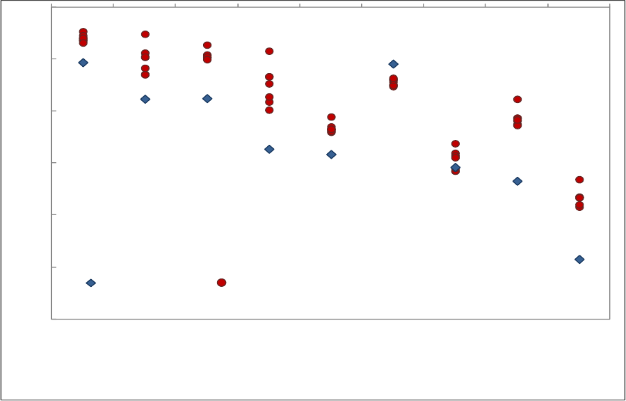
As shown in Figure 3, the model suggests that in some European periphery countries, bond
yield spreads (relative to Germany) exceeded their equilibrium value determined by long-run
and short-run fundamentals in the first half of 2012. The opposite picture emerges when
considering the case of several core euro area countries (e.g., Finland), where “safe haven”
effects result in spreads undershooting their equilibrium value. It is interesting to note the
contrasting results obtained for the pre-crisis period (1999-2009), during which the spreads in
European periphery countries were lower than the level justified by fundamentals. A similar
result on “underreaction” during 1999-2009 period and “overreaction” in the aftermath of the
crisis was obtained also in other recent studies (e.g., De Grauwe and Ji, 2012; Di Cesare and
et al., 2012). All in all, the model suggests that in some members of the euro area, current
sovereign borrowing costs deviate from the equilibrium level defined by macroeconomic
fundamentals. However, when interpreting these results one should bear in mind that they are
obtained form a very parsimonious model that does not account for some factors that likely
contributed to the temporary deviation of sovereign borrowing costs from their long-run
equilibrium level in the aftermath of the crisis (for instance, policy uncertainty).
14
V. CONCLUSIONS
This paper applies panel cointegration techniques to analyze long-run and short-run
determinants of government bond yields in 22 advanced economies during 1980-2010. The
employed methodology has several advantages over the techniques used in previous studies:
(i) it allows explicitly differentiating between long-run and short-run determinants of bond
yields; (ii) it pools long-run coefficients to improve efficiency and comply with theoretical
predictions, while maintaining flexibility in allowing country-specific variation of short-run
coefficients; and (iii) it allows testing for coefficient poolability.
Estimations suggest that in the long-run, government bond yields increase by about 2 basis
points in response to a 1 percentage point increase in the government debt-to-GDP ratio and
by about 45 basis points in response to a 1 percentage point increase in the potential growth
rate. In the short-run, changes in real bond yields deviate from their long-run equilibrium in
response to changes in the debt-to-GDP ratio (positive effect), real money market rates
(positive effect), and inflation (negative effect). The impact of changes in the growth rate
(negative effect) and the primary balance ratio (negative effect) is weaker. On average, about
half of the deviation from the long-run equilibrium is corrected within one year.
When applied to the current period, the model suggests that in some European periphery
countries, bond yield spreads (relative to Germany) in the first half of 2012 exceeded the
equilibrium value associated with long-run and short-run fundamentals. The opposite picture
emerges in the case of several core euro area countries (for example, Finland), where “safe-
haven” effects result in spreads undershooting their equilibrium value. All in all, the model
suggests that, in some members of the euro area, current sovereign borrowing costs deviate
from the equilibrium level defined by macroeconomic fundamentals.
Nevertheless, when interpreting these results, one should keep in mind that the analysis does
not account for some factors that likely contributed to the temporary deviation of sovereign
borrowing costs from their long-run equilibrium level in the aftermath of the crisis. These
include, for example, uncertainties related to the feedback effects between banks and
sovereigns and the contingent liabilities of the public sector. In addition, market overreaction
should not be interpreted as evidence against the effectiveness of fiscal adjustment to reduce
borrowing costs. A steady pace of fiscal adjustment remains imperative for anchoring lower
borrowing costs in the long run, while short-run departures of borrowing cost from the long-
run equilibrium should be addressed through complementary policies aimed at reducing
financial stress and market uncertainty.
15
REFERENCES
Ardagna, S., Caselli, F., and Lane, T. (2007), “Fiscal Discipline and the Cost of Public Debt
Service: Some Estimates for OECD Countries,” The B.E. Journal of
Macroeconomics, 7 (1): pp. 1-33.
Attinasi, M., Checherita, C., and Nickel, C. (2009), “What Explains the Surge in Euro Area
Sovereign Spreads During the Financial Crisis of 2007-09?” ECB Working Paper,
No. 1131 (Frankfurt: European Central Bank).
Baldacci, E., and Kumar, M. (2010), “Fiscal Deficits, Public Debt, and Sovereign Bond
Yields,” IMF Working Paper 10/184 (Washington: International Monetary Fund).
Bernoth, K., Von Hagen, J., and Schuknecht, L. (2012), “Sovereign Risk Premiums in the
European Government Bond Market,” Journal of International Money and Finance,
31: pp. 975-95.
Brook, A-M. (2003), “Recent and Prospective Trends in Real Long-Term Interest Rates,”
OECD Economics Department Working Paper No. 367 (Paris: Organization for
Economic Cooperation and Development).
Cebula, R. (2000), “Impact of Budget Deficits on Ex-Post Real Long-Term Interest Rates”,
Applied Economic Letters, 7: pp. 177-79.
Chinn, M. and Frankel, J. (2005), “The Euro Area and World Interest Rates”, Department of
Economics, University of California, Santa Cruz Working Paper No. 1031.
Conway, P. and Orr, A. (2002), “The GIRM: A Global Interest Rate Model”, Westpac
Institutional Bank Occasional Paper (Wellington: Westpac Institutional Bank).
De Grauwe, P. and Ji, Y. (2012), “Mispricing of Sovereign Risk and Multiple Equilibria in
the Eurozone”, CEPS Working Paper No. 361 (Leuven: Center for European Policy
Studies).
Di Cesare, A., Grande, G., Manna, M., and Taboga, M. (2012), “Recent Estimates of
Sovereign Risk Premia for Euro-Area Countries,” Banca D’Italia Occasional Paper
No. 128 (Rome: Banca D’Italia).
Elmendorf, D. (1993), “Actual Budget Deficit Expectations and Interest Rates”, Harvard
Institute of Economic Research Working Paper No. 1639.
Elmendorf, D. (1996), “The Effects of Deficit Reduction Laws on Real Interest Rates,”
Federal Reserve Board, Finance and Economics Discussion Series 1996–44.
Engen, E., and Hubbard, G. (2004), “Federal Government Debt and Interest Rates,” NBER
Working Paper No. 1068 (Cambridge, Massachusetts: National Bureau of Economic
Research).
Evans, P. (1987), “Interest Rates and Expected Future Budget Deficits in the U.S.,” Journal
of Political Economy, 95(1): pp. 34-58.
16
Faini, R. (2006), “Fiscal Policy and Interest Rates in Europe”, Economic Policy, July:
pp. 443–89.
Gale, W. and Orzsag, P. (2002), “The Economic Effects of Long-Term Fiscal Discipline”,
Tax Policy Center Discussion Paper, December.
Haugh, D., Ollivaud, P. and Turner, D. (2009), “What Drives Sovereign Risk Premiums? An
Analysis of Recent Evidence from the Euro Area”, OECD Economics Department
Working Paper No. 718 (Paris: Organization for Economic Cooperation and
Development).
Hauner, D. and Kumar, M. (2009), “Fiscal Policy and Interest Rates: How Sustainable is the
New Economy?” IMF Working Paper 06/112 (Washington: International Monetary
Fund).
Kinoshita, N. (2006), “Government Debt and Long-Term Interest Rate” IMF Working Paper
06/63 (Washington: International Monetary Fund).
Knot, K. and De Haan, J. (1995), “Fiscal Policy and Interest Rates in the European
Community”, European Journal of Political Economy, 11: pp. 171-87.
Laubach, T. (2009) “New Evidence on the Interest Rate Effects of Budget Deficits and
Debt,” Journal of European Economic Association, 7: pp. 858–85.
Lindé, J. (2001), “Fiscal Policy and Interest Rates in a Small Open Economy”, Finnish
Economic Papers, 14 (2): pp. 65-83.
Manasse, P., Roubini, N., and Schimmelpfennig, A. (2003), “Predicting Sovereign Debt
Crises,” IMF Working Paper 03/221 (Washington: International Monetary Fund).
Pesaran, H., Shin, Y., and Smith, R. (1999), “Pooled Mean Group Estimation of Dynamic
Heterogeneous Panels,” Journal of the American Statistical Association, 94: pp. 621-34.
Plosser, C. (1987), “Fiscal Policy and the Term Structure”, Journal of Monetary Economics,
Vol. 20 (2): pp. 343-67.
Schuknecht, L., von Hagen, J., Wolswijk, G. (2010), “Government Bond Risk Premiums in the
EU Revisited the Impact of the Financial Crisis”, ECB Working Paper No. 1152
(Frankfurt: European Central Bank).
Smith, P. and Wickens, M. (2002), “Macroeconomic Sources of FOREX Risk”, CEPR Working
Paper No. 3148 (London: Center for Economic Policy Research).
Thorbecke, W. (1993), “Why Deficit News Affects Interest Rates”, Journal of Policy Modeling,
15 (1): pp. 1-11.
Wachtel, P., and Young, J. (1987), “Deficit Announcements and Interest Rates”, American
Economic Review, 77: pp. 1007-22.

17
Table 1. Description of Variables and their Sources
Variable Description Expected sign Source
Dependent variable
Real long-term interest rate Nominal 10 year benchmark bond yield
(daily average) minus inflation divided over
one plus inflation*
Datastream
Long-run determinants
General government debt ratio Ratio of general government debt to GDP (in
percent)**
(+) WEO
Potential growth Real GDP growth filtered of cyclical
fluctuations
(+) WEO
Short-run determinants
Changes in debt ratio Ratio of general government debt to GDP (in
percent)**
(+)
Changes in inflation CPI inflation (+) WEO
Changes in real short-term interest rate Nominal 3 months money market rate (daily
average) minus inflation divided over one
plus inflation
(+) Datastream
Changes in output growth Real GDP growth (-) WEO
Changes in primary balance ratio Ratio of general government primary
balance to GDP
(-) WEO
Note: The sample covers the following advanced economies: Australia, Austria, Belgium, Canada, Denmark,
Finland, France, Germany, Greece, Iceland, Ireland, Italy, Japan, Korea, Netherlands, New Zealand, Portugal,
Spain, Sweden, Switzerland, the U.K., and the U.S.
*This is Fisher's formula, where inflation is calculated using the GDP deflator.
**Exceptions are Australia, Canada, Japan, and New Zealand, for which net debt-to-GDP ratio is used.

18
Table 2. Descriptive Statistics
Variable Obs Mean Std. Dev. Min Max
Real long-term interest rate
441 3.37 2.22 -4.06 10.98
General government debt ratio
441 57.63 28.59 -7.23 142.76
Inflation
441 2.37 1.60 -1.71 12.41
Real short-term interest rate
441 2.35 2.45 -3.52 14.42
Potential growth
441 2.54 1.42 -2.33 10.62
Primary balance ratio
441 -5.28 5.20 -35.16 4.16
Output growth
441 2.37 2.55 -8.23 10.92

19
Table 3. Panel Unit Root Tests
Test Null Alternative
hypothesis hypothesis Real interest
rate
Debt ratio Potential
growth
Im-Pesaran-Shin All panels contain
unit roots
Some panels are
stationary
0.000 0.949 0.000
Fischer All panels contain
unit roots
At least one panel is
stationary
0.015 0.528 0.000
Levin-Lin-Chu All panels contain
unit roots
All panels are
stationary
0.007 0.263 0.105
Breitung All panels contain
unit roots
All panels are
stationary
0.431 0.115 0.086
Hadri All panels are
stationary
Some panels contain
unit roots
0.000 0.000 0.000
P-value
Note: The panels include 22 advanced economies. The overall sample covers the 1980-2011 period. Some of
the tests require balanced panel and were applied to a balanced version of the dataset.

20
Table 4. Baseline Regressions
(1) (2) (3)
Full model Restricted
model
Adding EA
dummy
Long-run coefficients
Debt ratio 0.014** 0.021*** 0.025***
[0.006] [0.005] [0.005]
Potential growth 0.649*** 0.322** 0.393***
[0.143] [0.129] [0.114]
Debt ratio*Dummy_EA (1999-2009) -0.010** -0.020*** -0.016***
[0.005] [0.005] [0.005]
Potential growth*Dummy_EA (1999-2009) -0.763*** -0.395*** -0.359**
[0.128] [0.128] [0.160]
Constant 1.625*** 2.013*** 1.675***
[0.545] [0.477] [0.453]
Speed of adjustment -0.390*** -0.426*** -0.526***
[0.036] [0.034] [0.052]
Short-run coefficients
Debt ratio
0.091*** 0.081*** 0.092***
[0.027] [0.017] [0.020]
Inflation
-0.141** -0.159* -0.160**
[0.070] [0.086] [0.080]
Short-term real rate
0.151*** 0.135*** 0.124***
[0.044] [0.043] [0.040]
Dummy_EA (1999-2009) -0.248*
[0.134]
Output growth
0.007
[0.044]
Primary balance
-0.007
[0.056]
Obs. 441 441 441
Countries 22 22 22
AIC 1166.501 1268.079 1247.37
BIC 1211.481 1304.881 1288.26
Hausman p-value 0.893 0.902 0.644
St. Dev. of residuals 1.52 1.53 1.58
Note: Estimations are performed using the PMG estimator of Pesaran et al. (1999). The reported short-run
coefficients and the speed of adjustment are simple averages of country-specific coefficients. Robust standard
errors are in parentheses. ***, **, and * denote significance at 1, 5, and 10 percent confidence level,
respectively.

21
Table 5. Robustness Checks
(1) (2) (3) (4)
Excluding program
countries
Adding US
dummy
Adding JP
dummy
Using pre-crisis
sample
Long-run coefficients
Debt ratio 0.021*** 0.021*** 0.016** 0.012**
[0.005] [0.005] [0.007] [0.006]
Potential growth 0.527*** 0.328** 0.591*** 0.303**
[0.136] [0.135] [0.146] [0.144]
Debt ratio*Dummy_EA (1999-2009) -0.016*** -0.020*** -0.016*** -0.024***
[0.005] [0.005] [0.006] [0.006]
Potential growth*Dummy_EA (1999-2009) -0.487*** -0.395*** -0.434*** -0.381**
[0.133] [0.128] [0.154] [0.158]
Constant 1.511*** 2.003*** 1.483*** 2.566***
[0.498] [0.484] [0.521] [0.405]
Dummy_US -0.024
[0.272]
Dummy_Japan 0.798
[0.586]
Speed of adjustment -0.425*** -0.426*** -0.394*** -0.406***
[0.040] [0.034] [0.035] [0.062]
Short-run coefficients
Debt ratio
0.074*** 0.081*** 0.082*** 0.082***
[0.018] [0.017] [0.017] [0.020]
Inflation
-0.218** -0.158* -0.174** -0.127
[0.091] [0.086] [0.086] [0.091]
Short-term real rate
0.121*** 0.136*** 0.127*** 0.153***
[0.047] [0.043] [0.045] [0.045]
Obs. 390 441 441 388
Countries 19 22 22 22
AIC 1086.85 1270.07 1275.56 1035.02
BIC 1122.54 1310.96 1316.45 1070.67
Hausman p-value 0.93 0.94 1.00 0.47
St. Dev. of residuals 1.52 1.53 1.51 1.52
Note: Estimations are performed using the PMG estimator of Pesaran et al. (1999). The reported short-run
coefficients and the speed of adjustment are simple averages of country-specific coefficients. Robust standard
errors are in parentheses. ***, **, and * denote significance at 1, 5, and 10 percent confidence level,
respectively.

22
Figure 1. Selected Euro Area Economies: Real 10-Year Sovereign Bond Yields
(in percent)
-5.0
-2.5
0.0
2.5
5.0
7.5
10.0
12.5
15.0
17.5
20.0
1980
1981
1982
1983
1984
1985
1986
1987
1988
1989
1990
1991
1992
1993
1994
1995
1996
1997
1998
1999
2000
2001
2002
2003
2004
2005
2006
2007
2008
2009
2010
2011
Austria Belgium France Germany
Italy Netherlands Finland Greece
Ireland Portugal Spain

23
Figure 2. Selected Euro Area Economies: Debt-to-GDP Ratio
(in percent)
0.0
20.0
40.0
60.0
80.0
100.0
120.0
140.0
160.0
1980
1981
1982
1983
1984
1985
1986
1987
1988
1989
1990
1991
1992
1993
1994
1995
1996
1997
1998
1999
2000
2001
2002
2003
2004
2005
2006
2007
2008
2009
2010
2011
Austria Belgium France Germany
Italy Netherlands Finland Greece
Ireland Portugal Spain

24
Figure 3. Selected Euro Area Economies: Comparison of Predicted and Actual Long-
Run Real Bond Spreads vis-à-vis Germany
(first half of 2012)
-2
0
2
4
6
8
10
Austria
Belgium
France
Italy
Netherlands
Finland
Ireland
Portugal
Spain
Actual spread Model prediction
Note: reported are prediction results from seven models shown in tables 4-5. All spreads are calculated using
real bond yields.
25
Figure 4. Selected Euro Area Economies: Comparison of Predicted and Actual Long-
Run Real Bond Spreads vis-à-vis Germany
(1999-2009, average)
-3.0
-2.5
-2.0
-1.5
-1.0
-0.5
0.0
Austria
Belgium
France
Italy
Netherlands
Finland
Ireland
Portugal
Spain
Actual spread Model prediction
Note: reported are prediction results from seven models shown in tables 4-5. All spreads are calculated using
real bond yields.
