CH 204: Chemical Reaction Engineering - lecture
notes
January-April 2010
Department of Chemical Engineering
Indian Institute of Science
Bangalore 560 012
Contents
1 Introduction page 1
2 Review of background material 8
References 49
iii

1
Introduction
Levenspiel (2004, p. iii) has given a concise and apt description of chemical
reaction engineering (CRE):
Chemical reaction engineering is that engineering activity concerned with the ex-
ploitation of chemical reactions on a commercial scale. Its goal is the successful
design and operation of chemical reactors, and probably more than any other ac-
tivity, it sets chemical engineering apart as a distinct branch of the engineering
profession.
The ingredients of CRE are (i) thermodynamics, (ii) kinetics, (iii)
tranport processes, (iv) types of reactors, (v) mode of operation and con-
tacting, (vi) modelling and optimization, and (vii) control. These topics are
briefly discussed below.
1.1 Thermodynamics
1.1.1 Feasibility of the reaction
The standard free energy of formation ∆G
0
of gaseous NO at a temperature
T = 298 K and a reference pressure p
0
= 1 atm is 86.6 kJ/mol. Consider a
closed system that initially contains a mixture of N
2
and O
2
, and is main-
tained at a constant temperature T and a pressure p = p
0
. Consider the
reaction
1
2
N
2
(g) +
1
2
O
2
(g) NO(g) (1.1)
Here the notation “(g)” implies that the species is present in the gas phase.
Similarly, “(l)” and “(s)” will be used to denote species present in the liquid
and solid phases. respectively. Some NO will be formed by (1.1), but the
equilibrium mole fraction of NO (y
NO,e
) is 1 as ∆G
0
/(R T ) 1. Here R
1
2
is the gas constant, and y
NO,e
is the mole fraction attained at long times.
Hence we say that the reaction is not feasible under these conditions. The
conversion increases as T increases, but is less than 1 % even at T = 1780
K and p = 1 atm. Hence alternative reactions, such as the oxidation of NH
3
must be used to produce NO (Chatterjee and Joshi, 2008).
1.1.2 The heat of reaction
The sign of the heat of reaction ∆H determines whether the reactor should
be heated or cooled. The former applies for endothermic reactions (∆H >
0), and the latter for exothermic reactions (∆H < 0). The magnitude of
∆H determines the amount of heating or cooling required.
1.1.3 Allowance for thermodynamic non-idealities
For gaseous reactions at high pressure or low temperature, the equilibrium
constant K
p
, which is based on partial pressures, must be replaced by the
equilibrium constant K
f
, which is based on fugacities (Denbigh, 1971, p. 152,
see also section 2.8). For example, consider the ammonia synthesis reaction
N
2
(g) + 3 H
2
(g) 2 NH
3
(g) (1.2)
At T = 450
◦
C, the value of K
p
is 6.64 ×10
−3
at p = 10 atm and 8.84
×10
−3
at p = 300 atm (Denbigh, 1971, p. 152). Thus K
p
varies with the
pressure, whereas the value of K
f
is approximately constant in this pressure
range - it is 6.5 ×10
−3
at p = 10 atm and 6.6 ×10
−3
at p = 300 atm. The
slight variation of K
f
is caused by the use of approximate expressions for the
fugacities, based on the Lewis and Randall rule. Given the value of ∆G
0
, we
can calculate K
f
, and using the thermodynamic relations between fugacities
and partial pressures, the equilibrium composition can be calculated.
Similarly, for a liquid phase reaction involving the synthesis of methyl
tert-amyl ether (an additive for high octane gasoline) from methanol and
2-methyl-2-butene, the calculated activity coefficient for methanol is in the
range 6.4-7.7 at T = 298 K (Heintz et al., 2007).
1.2 Reactions and kinetics
1.2.1 Classification of reactions
Reactions may be classified by (a) the number of phases involved, (b) the
presence or absence of a catalyst, and (c) the nature of the overall reaction.

Introduction 3
If all the reactants and products, and catalysts, if any, are in a single
phase, the reaction is said to be homogeneous. An example is provided by
the thermal cracking of ethane to ethylene (Froment and Bischoff, 1990,
p. 29)
C
2
H
6
(g) C
2
H
4
(g) + H
2
(g) (1.3)
On the other hand, if more than one phase is involved, the reaction is said to
be heterogeneous. An example is provided by the chemical vapour deposition
(CVD) of Si on a substrate (Fogler, 1999, p. 675)
SiH
4
(g) → Si(s) + 2 H
2
(g) (1.4)
(silane)
Equation (1.3) represents a non-catalytic reaction, whereas ammonia
synthesis involves a solid catalyst. In some cases, a homogeneous catalyst
may be involved. For example, an enzyme called glucose isomerase catalyzes
the isomerization of glucose to fructose in the liquid phase (Fig. 1.1).
Fig. 1.1. Isomerization of glucose to fructose. Adapted from Schmidt (2005, p. 24).
Schmidt (2005, p. 24) notes that this is the largest bioprocess in the chemical
industry. As fructose is five times sweeter than glucose, the process is used
to make high-fructose corn syrup for the soft drink industries.
The overall reaction, as written, may represent either an elementary

4
reaction or a non-elementary reaction. An example of the former is given
by the gas-phase reaction (Laidler, 2007, p. 138)
NO
2
(g) + CO(g) NO(g) + CO
2
(g) (1.5)
Here NO is formed by the collision between molecules of NO
2
and CO, and
the rate expression conforms to the stoichiometry shown. On the other
hand, (1.4) represents a non-elementary reaction, as it actually proceeds by
the sequence of reactions shown below (Fogler, 1999, p. 666).
SiH
4
(g) SiH
2
(g) + H
2
(g)
SiH
2
(g) + ∗ → SiH
2
∗
SiH
2
∗ → Si(s) + H
2
(g) (1.6)
where * represents an active site on the substrate.
1.2.2 The rate expression
The rate expression provides information about the rate at which a reactant
is consumed. The rate is usually expressed per unit volume of the fluid for
fluid-phase reactions, and per unit area (or unit mass) of the catalyst for
reactions involving solid catalysts. For example, the rate of formation of Si
by the mechanism (1.6) is given by
˙r
Si
=
k p
SiH
4
p
H
2
+ K p
SiH
4
(1.7)
where p
SiH
4
and p
H
2
are the partial pressures of SiH
4
and H
2
, respectively.
Equation (1.7) can be derived from (1.6) by assuming that the reac-
tions follow mass action kinetics and invoking some other assumptions.
1.2.3 Alternative catalysts or alternative routes
The conventional process for the manufacture of 5-cyanovaleramide (an in-
termediate for a herbicide) by the hydrolysis of adiponitrile (Fig. 1.2) used
MgO as a catalyst (Pereira, 1999). The catalyst was difficult to recover and
reactivate, and the conversion had to be limited to 20 % to avoid a low
selectivity. An alternative process based on a supported enzyme catalyst
gave a high conversion and a high selectivity.

Introduction 5
Fig. 1.2. Conversion of adiponitrile to 5-cyanovaleramide.
1.3 Transport processes
1.3.1 Balance equations
For fluid-phase reactions, continuum equations are usually used. If the re-
actions involve two phases that are stratified, as in the case of a gas-liquid
reaction in a falling-film reactor, separate equations can be written for each
of the phases. If one phase is dispersed in the other, as in the case of stirred
liquid-liquid dispersions or fluidized beds, we can either write separate equa-
tions for each phase, or use some form of explicit or implicit averaging to
write continuum equations for each phase (see. for example, Jackson, 2000,
Yu et al., 2007).
1.3.2 Constitutive equations
For a fluid phase consisting of simple fluids such as air or water, the Navier-
Stokes equations are commonly used to describe momentum transfer, with
Fourier’s law for heat conduction. Diffusion is described either by Fick’s law
for binary mixtures, or by the Maxwell-Stefan equations for multicomponent
mixtures. For a stationary solid phase such as a bed of catalyst pellets, the
momentum balance is not required. However, Fourier’s law and Fick’s law
6
have to be modified by replacing the thermal conductivity and diffusivity by
the “effective” thermal conductivity and “effective” diffusivity, respectively.
For dispersed multiphase systems, constitutive equations are more
complicated, and not as firmly established as for single-phase systems.
1.4 Types of reactors
1.4.1 Ideal reactors
The adjective ideal refers to the state of mixing in the reactor. It is assumed
to be perfect in the case of ideal batch, semi-batch, and continuous stirred
tank reactors. The plug flow reactor corresponds to the assumption of perfect
mixing in the radial direction, no mixing in the axial direction, and a flat
axial velocity profile. As discussed in Levenspiel (2004, pp. 283-287, 321-
334) and Fogler (1999, pp. 873-876, 893-904) a sequence of ideal reactors
can sometimes be used to model nonideal reactors.
1.4.2 Actual reactors
In addition to the conventional stirred vessels, “empty” tubular reactors,
and packed beds, there are many other types of reactors such as fluidized
beds (Lee and Li, 2009), trickle beds (Wu et al., 2009), fluidized catalytic
crackers (Yang et al., 2009), bubble columns (Tokumura et al., 2009), mem-
brane reactors (Rahimpour and Ghader, 2004), microchannel reactors (Wang
et al., 2009), and multifunctional reactors (Fan et al., 2009; Agar, 1999). The
references in brackets represent recent articles discussing such reactors.
1.5 Mode of operation and contacting
Reactors can be operated either in batch, semi-batch or continuous modes.
The first two modes cause the concentrations of the species to vary with
time, whereas the latter can be operated in either a steady or unsteady
manner. Usually, startup, shutdown, and disturbances in feed flow rate, etc.
lead to unsteady operation. For some systems, it may be advantageous to
deliberately operate in an unsteady manner to achieve higher selectivity or
conversion. For example, Sotowa et al. (2008) examined the effect of forced
temperature cycling of a catalyst layer on propylene (C
3
H
6
) oxidation. They
found the forced operation led to a higher time-averaged conversion than
steady state operation, for the same rate of consumption of energy. The
Introduction 7
bombardier beetle provides an example of a natural system that relies on
forced periodic operation (Aneshansley et al., 1969).
For multiphase reactors, several modes of contacting, such as cocur-
rent, countercurrent, and cross-flow are possible. Gillou et al. (2008) ex-
amined the effect of introducing H
2
at various points along the length of
a microchannel reactor on the conversion of CO to hydrocarbons by the
Fischer-Tropsch process. Compared to the introduction of H
2
along with
CO at the inlet of the reactor, an increase in selectivity was obtained for
some hydrocarbons.
1.5.1 Modelling, control, and optimization
A mathematical model of the reactor permits prediction of the conversion,
selectivity (for systems with multiple reactions), flow patterns and hot spots
or regions of high temperature. The effect of changes in operating conditions
can also be examined. The availability of a model permits the development
of suitable control schemes to ensure product quality, and also provides a
valuable aid for the optimization of parameters or operating policies to sat-
isfy specific objective functions. For example, Altinten et al. (2008) modelled
a batch reactor used for the production of polystyrene. Using a suitable con-
trol scheme, the reactor temperature was varied with time so as to follow an
“optimum” profile. This ensured that a polymer of the desired molecular
weight was obtained in the minimum possible time.
2
Review of background material
2.1 Representation of reactions
The following notation will be used to represent irreversible and reversible
reactions:
A + B → C irreversible
A + B C reversible (2.1)
Let A
i
, i = 1, N represent N species participating in a single reaction
a
1
A
1
+ a
2
A
2
+ ... a
m
A
m
+ ...a
N
A
N
where a
i
represents the number of moles of species A
i
. The reaction can be
written compactly as
Σ
N
i=1
ν
j
A
j
= 0
where ν
j
is the stoichiometric coefficient for A
j
. The usual convention is
v
j
< 0, for reactants; v
j
> 0, for products
For a reversible reaction, a species may be either a product or a reactant,
depending on the direction in which the reaction proceeds. In such a case,
the signs for the ν
i
are chosen in the usual manner, i.e. assuming that the
reaction proceeds from left to right. In case the reaction proceeds in the
opposite direction, the expression for the reaction rate will change sign and
the signs of the ν
j
can be left unchanged.
The above notation can be readily extended to multiple reactions.
If N species participate in M reactions, the reactions can be represented by
N
X
j=1
ν
ij
A
j
= 0, i = 1, M
8

Review of background material 9
where ν
ij
is the stoichiometric coefficient for the j
th
species participating in
the i
th
reaction.
2.2 The condition for reaction equilibrium
Consider an isolated system in which the reaction A
1
+ A
2
A
3
occurs.
(An isolated system is one that does not interact with its surroundings. In
particular, there is no transfer of heat, mass, or work between the system
and the surroundings.) The second law of thermodynamics states that all
changes or processes occurring in an isolated system must satisfy
dS
dt
≥ 0 (2.2)
where S is the total entropy of the system and t is the time. The system is
said to be at an equilibrium state if
dS
dt
= 0
If we start with a binary mixture of A
1
and A
2
, A
3
will be produced
as the reaction proceeds. In accord with (2.2), S must either increase or
remain constant. The expected variation of the entropy S and the molar
concentration c
1
of A
1
with t is sketched in Fig. 2.1. The quantities S
e
and
C
1e
represent the equilibrium values of S and C
1
, respectively.
It follows from the above discussion that S is a maximum at an
equilibrium state of an isolated system. In thermodynamics, an isolated
system is defined as one that has a constant volume V and a constant
internal energy U. Hence the equilibrium state corresponds to one that
implies a maximum of S at constant U and V .
In reaction engineering, it is convenient to work with a closed system,
rather than an isolated system. (A closed system is one that does not
exchange mass with the surroundings.) We shall now derive the condition for
the equilibrium state of a closed system in terms of a suitable thermodynamic
quantities. The material below has been adapted from Denbigh (1971, p. 67-
69).
Consider a closed system in contact with a heat reservoir that is
maintained at a constant temperature T
r
. Treating the system and the
reservoir as an isolated compound system, the second law implies that
∆S + ∆S
r
≥ 0 (2.3)
where ∆S and ∆S
r
are the entropy changes of the system and the reservoir,

10
Fig. 2.1. Variation of the total entropy of the system S and the concentration of
species 1 c
1
with the time t in an isolated system. The quantities S
e
and c
1e
represent the equilibrium values of S and c
1
, respectively.
respectively. If ∆Q is the heat absorbed by the system from the reservoir,
we have
∆S
r
= −(∆Q)/T
r
(2.4)
regardless of whether the heat transfer is reversible or irreversible. The first
law of thermodynamics implies that
∆U = ∆Q − ∆W (2.5)
where ∆U is the change in internal energy of the system and ∆W is the

Review of background material 11
work done by the system on the surroundings. Equations (2.3)-(2.5) imply
that
T
r
∆S − (∆U + ∆W ) ≥ 0
or, adding and subtracting ∆(p V ), where p is the pressure of the fluid
∆(U + p V − T
r
S) ≤ −∆W + ∆(p V ) (2.6)
Consider a special case where the initial state 1 and the final state
2 of the system are such that (i) T
1
= T
2
= T
r
≡ T , and (ii) p
1
= p
2
≡ p.
Noting that the Gibbs free energy is defined by
G ≡ U + p V − T S (2.7)
(2.6) reduces to
∆G|
T,p
≤ −(∆W − p ∆V ) ≡ −∆W
0
(2.8)
where ∆W
0
is the work done by the system, excluding that due to volume
change. (For a solid phase, the work due to volume change is not given by
p ∆V . However, the final result (2.9) is unaltered (Callen, 1985, p. 305).)
If ∆W
0
= 0, (2.8) reduces to
∆G|
T,p
≤ 0 (2.9)
Hence the Gibbs free energy G must either remain constant or decrease for
all changes in a closed system maintained at constant T, p, and G must be
a minimum at equilibrium.
In order to relate (2.9) to measurable quantities such as temperature,
pressure, and composition, we use the Gibbs equation. For a single-phase
system containing N species, the Gibbs equation is given by
dG = V dp −S dT +
N
X
i=1
µ
i
dn
i
(2.10)
where
µ
i
≡
∂G
∂n
i
T, p, n
j6=i
(2.11)
is the chemical potential of species i, and n
i
is the number of moles of species
i.
Consider a single reaction occurring in a closed system containing a

12
fluid, and assume that there are no spatial gradients. Then the mass balances
are given by
dn
i
dt
= V ν
i
˙r, i = 1, N (2.12)
where V is the volume of the system and ˙r is the reaction rate for this
reaction. For fluid-phase systems, the usual dimensions of ˙r are moles/unit
volume/unit time. Even though there are N equations of the form (2.12),
there is only one independent reaction. Hence, as suggested by de Donder
(1922) (cited in Laidler, 2007, p. 7), all the {n
i
} can be expressed in terms
of a variable ξ, called the extent of reaction. Let
n
i
= n
i0
+ ν
i
ξ, i = 1, N (2.13)
where n
i0
is the initial (i.e. at time t = 0) number of moles of i. Equations
(2.13) and (2.12) imply that
dξ
dt
= V ˙r (2.14)
with the initial condition ξ(0) = 0.
Expressing the mole numbers in terms of the extent of reaction,
(2.10) can be written as
dG = V dp −S dT +
N
X
i=1
µ
i
ν
i
dξ (2.15)
As G must be a minimum at an equilibrium state of a closed system main-
tained at constant (T, p), we must have
∂G
∂ξ
T,p
= 0
or
N
X
i=1
µ
i
ν
i
= 0 (2.16)
and
∂
2
G
∂ξ
2
T,p
> 0
or
N
X
i=1
∂µ
i
∂ξ
T,p
ν
i
> 0 (2.17)
Equation (2.16) represents the condition for reaction equilibrium. It

Review of background material 13
holds even if the system contains more than one phase, and the reaction
involves components in different phases (Denbigh, 1971, p. 140).
The affinity of the reaction is defined by
˜
A ≡ −
N
X
i=1
µ
i
ν
i
(2.18)
Equation (2.15) implies that
∂G
∂ξ
T,p
= −
˜
A (2.19)
Hence if
˜
A > 0, G decreases as the extent of reaction ξ increases, and the
reaction proceeds from left to right.
2.3 Models for the chemical potential
Equation (2.15) can be used to compute the equilibrium composition for
a single reaction in a closed system, provided a model is available for the
dependence of the chemical potentials {µ
i
} on temperature T , pressure p,
and composition. Some models are discussed briefly below. For more details,
the reader is referred to Denbigh (1971, pp. 111-115, 125-126, 249, 270-271)
and Smith et al. (2001, pp. 384, 390, 577).
(a) The perfect gas mixture
The perfect gas mixture is defined as one for which (Denbigh, 1971,
p. 115)
µ
i
(T, p, y) ≡ µ
i0
(T, p
0
) + R T ln
p y
i
p
0
, i = 1, N (2.20)
where y is the vector of N − 1 independent mole fractions y
i
, i = 1, N − 1,
µ
i0
is the chemical potential of pure i at a temperature T and a reference
pressure p
0
, R is the gas constant, y
i
is the mole fraction of species i, and
p is the total pressure of the mixture. The use of (2.20) along with suitable
thermodynamic relations leads to the following familiar results for a perfect
gas mixture
p V = n R T ; p
i
≡ p y
i
= n
i
R T/V, i = 1, N (2.21)
where V is the volume occupied by the mixture, p
i
is the partial pressure of
14
i, n
i
is the number of moles of species i, and
n ≡
N
X
i=1
n
i
is the total number of moles.
(b) The ideal solution
The ideal solution is defined by (Denbigh, 1971, p. 249)
µ
i
(T, p, y) ≡ µ
i0
(T, p) + R T ln(y
i
), i = 1, N (2.22)
where µ
i0
is the chemical potential of pure i at (T, p). Equation (2.22) can
be used for ideal gaseous, liquid, or solid solution.
(c) The non-ideal solution
To account for non-ideal behaviour, (2.22) is modified by introducing
a variable γ
i
, called the activity coefficient, such that (Denbigh, 1971, p. 270)
µ
i
(T, p, y) ≡ µ
i0
(T, p) + R T ln(γ
i
y
i
), i = 1, N (2.23)
Note that µ
i0
is independent of the composition, and the composition de-
pendence of µ
i
is accounted for solely by the term γ
i
y
i
. The value of µ
i0
can be fixed by choosing a convention for γ
i
. If all the species forming the
solution remain in the same phase as the solution in their pure states at
(T, p), the usual convention is
γ
i
→ 1 as y
i
→ 1 (2.24)
In this case, µ
i0
is the chemical potential of pure i at (T, p).
Consider a liquid solution, and let i = 1, m denote species that re-
main as liquids in their pure states at (T, p). The other species (i = m+1, N)
are either gases or solids in their pure states at (T, p). Convention (2.24)
applies to the first m species, and hence
γ
i
→ 1 as y
i
→ 1, i = 1, m (2.25)
For the other species, the usual convention is
γ
i
→ 1 as y
i
→ 0, i = m + 1, N (2.26)
For i = m + 1, N , µ
i0
is the chemical potential of pure i in a hypothetical
liquid state. It is a hypothetical state as pure i will not, by definition, be in
a liquid state at (T, p).
Equation (2.23) can be used for gaseous, liquid, or solid solutions.

Review of background material 15
Additional details regarding the determination and use of activity coeffi-
cients may be found in Denbigh (1971, pp. 281-288), Prausnitz et al. (1999,
pp. 222-236), and Sandler (2006, pp. 419-461).
Remarks
1. The activity of a species i is defined by Denbigh (1971, p. 287)
a
i(y)
≡ γ
i
y
i
(2.27)
where the subscript y indicates that mole fractions are used as a measure of
the composition of the mixture, and γ
i
is the activity coefficient based on
mole fractions. For some applications, it is convenient to replace y
i
in (2.27)
by some other measures of the composition, such as the molar concentration
c
i
or the molality ˆc
i
. Here ˆc
i
is the number of moles of i per kg of the solvent.
The molality is often used for electrolyte solutions (Prausnitz et al., 1999,
p. 218).
Thus we have
a
i(c)
≡
γ
i(c)
c
i
c
i0
a
i(ˆc)
≡
γ
i(ˆc)
ˆc
i
ˆc
i0
(2.28)
As the activity is a dimensionless quantity, (2.28) involve a reference compo-
sition characterized by c
i0
or ˆc
i0
. For ions and molecules dissolved in water,
the usual reference composition is (Sawyer et al., 2003, p. 31, Sandler, 2006,
p. 712)
c
i0
= 1 M (i.e. 1 mol/L), ˆc
i0
= 1 mol/kg of water (2.29)
For the solvent, and for pure liquids and solids in equilibrium with an aque-
ous solution, the usual reference state is the concentration or molality of the
pure component
c
i0
= c
i, pure
; ˆc
i0
= ˆc
i, pure
(2.30)
The conventions adopted for γ
i(c)
and γ
i(ˆc)
are similar to those used for γ
i
.
For example, consider a liquid mixture and a solute i that is not a liquid at
the same (T, p) as the solution. Then the convention is that
γ
i(c)
→ 1 as c
i
→ 0 (2.31)
In terms of the activities, (2.23) can be rewritten as
µ
i
≡ µ
i0
(T, p) + R T ln a
i(y)
(2.32)
≡ µ
i0(c)
(T, p) + R T ln a
i(c)
(2.33)

16
≡ µ
i0(ˆc)
(T, p) + R T ln a
i(ˆc)
(2.34)
2. For gas mixtures, it is common practice to use fugacities instead of
activity coefficients. Thus (2.23) can be rewritten as Denbigh (1971, p. 125)
µ
i
(T, p, y) ≡ µ
i0
(T, p
0
) + R T ln
f
i
f
i0
, i = 1, N (2.35)
where f
i
is the fugacity of species i and µ
i0
and f
i0
are the chemical potential
and fugacity, respectively, of pure i at a temperature T and a reference
pressure p
0
. A common choice for f
i0
is f
i0
(T, p
0
) = 1 atm, in which case
p
0
is the pressure for which the fugacity of pure i is 1 atm. As noted by
Denbigh (1971, p. 123), if p ≤ 1 atm, f
i0
≈ p
0
for most gases. Thus the
choice f
i0
= 1 atm implies that p
0
≈ 1 atm.
As in the case of (2.23), (2.35) can be used for gaseous, liquid, and
solid solutions.
3. In accord with the experimental observation that the mixture should
behave like a perfect gas mixture in the limit p → 0, (2.20) and (2.35) imply
that
lim
p→0
f
i
f
i0
=
p y
i
p
0
(2.36)
Thus the fugacity is proportional to the partial pressure p
i
≡ p y
i
at low
pressures.
4. For an ideal solution, (2.22) and (2.35) imply that
R T ln
f
i
f
i0
y
i
= µ
i0
(T, p) −µ
i0
(T, p
0
) (2.37)
As the right hand side is independent of the composition, its value remains
unchanged in the limit y
i
→ 1. Hence (2.37) implies that
f
i
f
i0
y
i
= lim
y
i
→1
f
i
f
i0
y
i
=
f
i,pure
f
i0
or
f
i
= f
i,pure
y
i
(2.38)
Equation (2.38) is called the Lewis and Randall rule.

Review of background material 17
2.4 The equilibrium constant and the equilibrium composition
For a single reaction in a single phase system, the condition for reaction
equilibrium is (see (2.17))
N
X
i=1
µ
i
ν
i
= 0 (2.39)
For a perfect gas mixture, (2.39) and (2.20) imply that
N
X
i=1
µ
i0
ν
i
= −R T ln
"
N
Y
i=1
p
ie
p
0
ν
i
#
(2.40)
where p
ie
is the equilibrium value of the partial pressure p
i
of species i. The
equilibrium constant is defined by
K
p
≡
N
Y
i=1
p
ie
p
0
ν
i
=
N
Y
i=1
p y
ie
p
0
ν
i
(2.41)
where y
ie
is equilibrium mole fraction of species i. Introducing the standard
Gibbs free energy change for the reaction
∆G
0
≡
N
X
i=1
µ
i0
(T, p
)
) ν
i
(2.42)
(2.40) can be rewritten as
∆G
0
−R T ln K
p
(2.43)
Equations (2.42) and (??) imply that K
p
is independent of the pressure p
and K
p
= K
p
(T ). This is true only for a perfect gas mixture. For a non-ideal
gas mixture, K
p
is still defined by (2.41), but (2.43) is not valid.
The equilibrium composition in a closed system at constant (T, p)
can be calculated as follows. For ease of discussion, consider a perfect gas
mixture. Using tables of thermodynamic properties, values of ∆G
0
can be
calculated for most reactions. The value of K
p
then follows from (2.43). As
y
ie
= n
ie
/n
e
(2.44)
where n
ie
and n
e
are the number of moles of species i and the total number
of moles, respectively, at equilibrium, (2.41) can be rewritten as
K
p
=
N
Y
i=1
p n
ie
p
0
n
e
ν
i
(2.45)

18
or using (2.13)
K
p
=
N
Y
i=1
p
p
0
n
i0
+ ν
i
ξ
e
n
0
+ (∆ν) ξ
e
ν
i
(2.46)
Here ξ
e
is the extent of reaction at an equilibrium state, and n
0
≡
P
N
i=1
n
i
and ∆ν ≡
P
N
i=1
ν
i
are the total number of moles at the initial state and
the change in the number of moles accompanying the reaction, respectively.
Equation (2.46) represents a nonlinear equation for the extent of reaction
ξ
e
. Except in simple cases, the equation must be solved iteratively.
2.5 The effect of temperature on the equilibrium composition of
a perfect gas mixture
Taking the logarithm of (2.45) and using (2.43), we obtain
−
∆G
0
R T
= ln K
p
=
N
X
i=1
ν
i
ln
p n
ie
p
0
n
e
(2.47)
Differentiating (2.47) with respect to T , and using (2.13), we obtain
d
dT
−
∆G
0
R T
=
d
dT
(ln K
p
) =
N
X
i=1
ν
i
n
ie
dn
ie
dξ
e
−
ν
i
n
e
dn
e
dξ
e
dξ
e
dT
(2.48)
Substituting for ∆G
0
from (2.42), we obtain
d
dT
−
∆G
0
R T
== −
N
X
i=1
ν
i
R
d
dT
µ
i0
T
=
∆H
0
R T
2
(2.49)
where
∆H
0
≡
N
X
i=1
ν
i
h
i0
(2.50)
is the standard enthaply change for the reaction and h
i0
is the molar enthalpy
of pure i at (T, p
0
). Hence (2.48) reduces to van’t Hoff’s equation
d
dT
(ln K
p
) =
∆H
0
R T
2
(2.51)
As n
i
= n
i
(ξ), (2.13) and (2.48) imply that
d
dT
(ln K
p
) =
"
N
X
i=1
ν
2
i
n
ie
−
(∆ν)
2
n
e
#
dξ
e
dT
(2.52)

Review of background material 19
Using (2.52), (2.51) can be rewritten as
∆H
0
R T
2
=
"
N
X
i=1
ν
2
i
n
ie
−
(∆ν)
2
n
e
#
dξ
e
dT
(2.53)
The Schwarz inequality (see, for example, Arfken and Weber, 2001, p. 607)
can be used to show that the quantity in square brackets on the right hand
side of (2.53) is always positive. Hence dξ
e
/dT has the same sign as ∆H
0
.
An exothermic reaction is defined as one for which ∆H
0
< 0. In this
case, dξ
e
/dT < 0, and hence the equilibrium extent of reaction decreases as
T increases. If species i is a reactant, its conversion X
i
, defined by
X
i
≡
n
i0
−n
i
n
i0
(2.54)
is directly proportional to the extent of reaction ξ. Hence X
i
also decreases
as T increases. Conversely, for an endothermic reaction, the equilibrium
conversion increases as T increases.
Remark Consider a chemical reaction in closed system, whose volume V
changes suitably to maintain constant (T, p). If the state of the system
changes from state 1 to state 2 as the reaction proceeds, the enthalpy change
of the system is given by
∆H = ∆U + ∆(p V ) = ∆U + p ∆V
or, using the first law of thermodynamics, and assuming that work is asso-
ciated only with volume change
∆H = ∆Q (2.55)
where ∆Q is the heat absorbed by the system. Thus ∆H
0
is the heat
absorbed by the system when the reactants are taken in stoichiometric pro-
portions, with each reactant at (T, p
0
), and are completely converted to
products, with each product at (T, p
0
) (Denbigh, 1971, p. 142).
2.6 The effect of pressure on the equilibrium composition of a
perfect gas mixture
Differentiating (2.47) with respect to p, we obtain
∂
∂p
(ln K
p
) = 0 =
"
N
X
i=1
ν
2
i
n
ie
−
(∆ν)
2
n
e
#
∂ξ
e
∂p
+
∆ν
p

20
or
∂ξ
e
∂p
= −
∆ν
p
h
P
N
i=1
ν
2
i
n
ie
−
(∆ν)
2
n
e
i
(2.56)
If the reaction is accompanied by an increase in the number of moles, i.e.,
∆ν > 0, (2.56) implies that ∂ξ
e
/∂p < 0. Hence the equilibrium conversion
decreases as p increases. Conversely, if ∆ν > 0, the conversion increases as
p increases.
Remark Equations (2.53) and (2.56) are quantitative expressions of Le Chate-
lier’s principle (Atkins and de Paula, 2002, p. 234): “A system at equilib-
rium, when subjected to a disturbance, responds in a way that tends to
minimize the effect of the disturbance.”
2.7 Feasibility of reactions
As mentioned in section 2.2, a reaction proceeds from left to right if
˜
A = −
N
X
i=1
µ
i
ν
i
> 0
The computation of
˜
A requires a knowledge of T, p, and the composition.
A rough idea of the direction in which the reaction is likely to occur may
be obtained by calculating the standard free energy change for the reaction
∆G
0
=
P
N
i=1
µ
i0
(T, p
0
) ν
i
. Large negative values of ∆G
0
imply that the
reaction is promising, i.e. it is likely to proceed from left to right. On
the other hand, large positive values of ∆G
0
imply that the reaction is not
promising, i.e. it is likely to proceed from right to left.
Equation (2.43) implies that if ∆G
0
0, K
p
is 1. To understand
the effect of K
p
on the conversion, it is helpful to rewrite (2.46) as
ln K
p
= q ≡
N
X
i=1
ν
i
[ln(n
i0
+ ν
i
ξ
e
) −ln(n
0
+ (∆ν) ξ
e
)] + (∆ν) ln(p/p
0
) (2.57)
At a fixed value of p, if K
p
increases, (2.57) implies that ξ
e
increases, as
∂q/∂ξ
e
> 0. Conversely, if K
p
1, we may expect ξ
e
to be small. However,
if the initial mixture contains only the reactants, the equilibrium value of ξ
e
will be small but non-zero even if ∆G
0
0.
Dodge (1944) has listed the following thumb rules: (a) if ∆G
0
(298
K, 1 atm) < 0, the reaction is promising, (b) if 0 < ∆G
0
< 40 kJ/mol, a
more detailed examination is warranted, and (c) if ∆G
0
> 40 kJ/mol, the

Review of background material 21
reaction is very unlikely. For example, consider the synthesis of NO from
N
2
and O
2
. For this reaction, ∆G
0
= 86.6 kJ/mol of NO, whereas for the
synthesis of NH
3
by the reaction
1
2
N
2
(g) +
3
2
H
2
(g) NH
3
(g) (2.58)
∆G
0
= −17 kJ/mol of NH
3
. Hence the thumb rules suggest that very little
NO will be formed.
2.8 Reaction equilibrium in an imperfect gas mixture
Using the model (2.35) for the chemical potential and the condition for
reaction equilibrium (2.16), we obtain
N
X
i=1
µ
i
ν
i
= 0
or
R T ln K
f
= −∆G
0
(T, p
0
) (2.59)
where
K
f
≡
N
Y
i=1
f
ie
f
i0
ν
i
(2.60)
is the equilibrium constant based on fugacities and f
ie
is the equilibrium
value of the fugacity of species i.
For an imperfect gas mixture, it is K
f
and not K
p
that is independent
of the pressure p. This point is illustrated by the data of Larson and Dodge
(cited in Denbigh, 1971, p. 152). As p increases from 10 atm to 300 atm,
K
p
increases by 34 % of the smaller value, whereas K
f
increases by only 1.5
%. The small variation of K
f
occurs because of the errors introduced by
using the Lewis and Randall rule (2.38) to estimate the fugacities {f
i
}. For
p > 300 atm, the variation of K
f
is more pronounced.
2.9 Reaction equilibrium in a liquid mixture
If (2.23) is used as a model for the chemical potential, (2.39)implies that
N
X
i=1
µ
i0
ν
i
= −R T ln K
γ
K
y
(2.61)
22
where
K
γ
≡
N
Y
i=1
γ
ν
i
i
; K
y
≡
N
Y
i=1
y
ν
i
i
(2.62)
Equation (2.61) can be used to calculate the equilibrium composition
provided the values of the {µ
i0
} are known. For solutes that are not liquids
at the same (T, p) as the solution, (2.26), (2.27), and (2.32) imply that µ
i0
is
the chemical potential of pure i in a hypothetical liquid state. However, the
values tabulated for such solutes often correspond to a hypothetical ideal
solution of unit molality. In such cases, activities defined on the molality
scale may be used. Equations (2.34) and (2.29) imply that µ
i0(ˆc)
(T, p) is the
chemical potential of i in a hypothetical ideal solution of unit molality. Fur-
ther, as noted by Denbigh (1971, p. 294), the effect of pressure on the liquid
and solid phases may usally be neglected, unless it is very high compared to
the standard pressure p
0
= 1 atm. Hence
µ
i0(ˆc)
(T, p) ≈ µ
i0(ˆc)
(T, p
0
) (2.63)
and the tabulated value of the standard Gibbs free energy of formation of i
may be used for µ
i0(ˆc)
(T, p).
2.10 Reaction equilibrium in systems involving multiple phases
Consider the thermal decomposition of caclium carbonate (Denbigh, 1971,
p. 156)
CaCO
3
(s) CaO (s) + CO
2
(g) (2.64)
The partial pressure of CO
2
, p
CO
2
can be related to the standard Gibbs free
energy change for the reaction as follows.
The condition for reaction equilibrium is
−µ
CaCO
3
(s) + µ
CaO
(s) + µ
CO
2
(g) = 0 (2.65)
Assuming that both CaCO
3
(s) and CaO (s) have negligible vapour pres-
sures, only CO
2
will be present in the vapour phase. Treating it as a perfect
gas, we have
µ
CO
2
(g) = µ
0,CO
2
(T, p
0
) + R T ln(p
CO
2
/p
0
) (2.66)
Using (2.66), (2.67) reduces to
−µ
CaCO
3
(s) + µ
CaO
(s) + µ
0,CO
2
(g) = −R T ln(p
CO
2
/p
0
) (2.67)

Review of background material 23
To proceed further, we assume that CaCO
3
(s) and CaO (s) form
immiscible solid phases, i.e. a phase contains either pure CaCO
3
or pure
CaO. (The case where two solids are miscible and form a mixture or solid
solution is discussed in Sandler (2006, pp. 679-687).) Then µ
CaCO
3
and µ
CaO
depend only on (T, p). For a pure phase, dµ = −s dT + v dp, where s and v
are the molar entropy and the molar volume, respectively, of the material.
Considering CaO and assuming that v
CaO
is approximately independent of
p, we obtain
µ
CaO
(T, p) = µ
CaO
(T, p
0
) + v
CaO
(p −p
0
) (2.68)
Using a similar expression for µ
CaCO
3
,
µ
0,CaO (s)
(T, p
0
) + µ
0,CO
2
(g)
(T, p
0
) − µ
0,CaCO
3
(s)
(T, p
0
)
+(v
CaO (s)
− v
CaCO
3
(s)
) (p − p
0
) = −R T ln(p
CO
2
/p
0
) (2.69)
As
∆G
0
= µ
0,CaO (s)
(T, p
0
) + µ
0,CO
2
(g)
(T, p
0
) − µ
0,CaCO
3
(s)
(T, p
0
) (2.70)
(2.69) reduces to
∆G
0
+ (v
CaO (s)
− v
CaCO
3
(s)
) (p − p
0
) = −R T ln(p
CO
2
/p
0
) (2.71)
The second term on the left hand side of (2.71) is usually negligible
compared to the first term. For example, ∆G
0
(298K, 1atm) = 135 kJ/mol,
whereas (v
CaO (s)
− v
CaCO
3
(s)
) (p − p
0
) ≈ 0.2 kJ/mol for p − p
0
= 100 atm.
Hence (2.71) may be approximated as
∆G
0
≈ −R T ln(p
CO
2
/p
0
) (2.72)
By analogy with (2.41), we may define a partial equilibrium constant
K
0
p
≡
p
CO
2
p
0
(2.73)
Equation (2.72) permits evaluation of the pressure of CO
2
(g) that is in
equilibrium with CaCO
3
(s) and CaO (s). As noted by Denbigh (1971,
p. 158), if p
CO
2
/p
0
> K
0
p
, CaO will be converted to CaCO
3
.
Another example involving gaseous and liquid phases is given by the
formation of urea by the reaction (Denbigh, 1971, p. 294)
CO
2
(g) + 2 NH
3
CO(NH
2
)
2
(aq) + H
2
O (2.74)
Numbering the species from left to right in the above equation as 1-4, the

24
values reported in the literature for the standard free energies of formation
are, in kJ/mol
µ
10
= −394.4, µ
20
= −16.64, µ
30(ˆc)
= −203.8, µ
40(y)
= −237.2 (2.75)
Hence the standard free energy change for the reaction (2.75) is
∆G
0
≡ µ
40(y)
+ µ
30(ˆc)
− 2 µ
20
− µ
10
= −13.32 kJ/mol (2.76)
and the condition for reaction equilibrium is
∆G
0
= −R T ln
γ
4
x
4
γ
3(ˆc)
(ˆc
3
/ˆc
30
)
(f
2
/f
20
)
2
(f
1
/f
10
)
(2.77)
2.11 Systems with multiple reactions
The discussion will be confined to a single phase system containing N species
participating in M reactions. For example. the following reactions occur
during the production of formaldehyde (HCHO) from methanol (CH
3
OH):
CH
3
OH HCHO + H
2
CH
3
OH +
1
2
O
2
HCHO + H
2
O
HCHO CO + H
2
HCHO +
1
2
O
2
CO + H
2
O
CO +
1
2
O
2
CO
2
(2.78)
We could also add the reaction
CH
3
OH CO + 2 H
2
but it is not an independent reaction, as it can be obtained by adding the
first and the third reactions in (2.78).
It is useful to calculate the number of stoichiometrically independent
reactions N
R
. The value of N
R
permits examination of a system involving
N
R
reactions, rather than the original system of M ≥ N
R
reactions. A
method for calculating N
R
is explained below.
Consider the system of reactions
N
X
j=1
ν
ij
A
j
= 0, i = 1, M (2.79)
Review of background material 25
where ν
ij
is the stoichiometric coefficient for the j
th
species in the i
th
reac-
tion. Let the stoichiometric matrix [ν ] be defined by
[ν ] = [ν
ij
] (2.80)
Thus the element in the i
th
row and j
th
column of [ν ] is ν
ij
. The number
of stoichiometrically independent reactions is given by
N
R
= rank([ν ]) (2.81)
Here the rank of [ ν ] is the maximum number of linearly independent rows
or columns of [ ν ] (Kreyszig, 1993, p. 356-357); it can be found by Gaussian
elimination or Gauss elimination, as discussed in Aris (1999, p. 13) and in
books on numerical analysis (see, for example, Gerald and Wheatley, 1994,
pp. 113-115). The following example is taken from Aris (1999, pp. 13-14).
Consider the reactions involved in the formation of hydrogen bromide
(HBr):
Br
2
→ 2 Br
Br + H
2
→ HBr + H
H + Br
2
→ HBr + Br
H + HBr → H
2
+ Br
2 Br → Br
2
(2.82)
The stoichiometric matrix is given by
ν =
−1 2 0 0 0
0 −1 −1 1 1
−1 1 0 1 −1
0 1 1 −1 −1
1 −2 0 0 0
The procedure is as follows.
(i) Rearrange the rows if necessary, so that the pivot ν
11
6= 0. In the
present example, rearrangement is not required.
(ii) Divide the first row by ν
11
so that the first row is now given by
ν
1j
= [1 − 2 0 0 0].
(iii) Using row operations, i.e. forming linear combinations of the other
rows with the first row, make all the elements in the first column
26
(except ν
11
) equal to zero. Thus we obtain
ν
0
=
1 −2 0 0 0
0 −1 −1 1 1
0 −1 0 −1 1
0 1 1 −1 −1
0 0 0 0 0
(iv) Repeat steps 1-3, starting with ν
22
as the pivot, and reducing ν
i2
, i =
3, N to zero. The result is
ν =
1 −2 0 0 0
0 1 1 −1 −1
0 0 1 −2 0
0 0 0 0 0
0 0 0 0 0
As all the elements in the 3rd and 4th rows are zero, the process can
be stopped at this stage. The rank of ν is 3, the number of non-zero rows.
Hence (2.81) implies that the number of stoichiometrically independent re-
actions is N
R
= 3 in the present example.
2.12 Degrees of freedom for reactive systems
Suppose there are N species, P phases, and N
R
independent chemical reac-
tions. At an equilibrium state, the following conditions hold (Denbigh, 1971,
p. 187):
T
j
= T
1
; p
j
= p
1
; µ
ji
= µ
1i
, j = 2, P ; i = 1, N (2.83)
Here T
j
and p
j
are the temperature and pressure, respectively, of phase j
and µ
ji
is the chemical potential of species i in phase j. In addition, there
are N
R
conditions of reaction equilibrium, given by
N
X
i=1
ν
li
µ
1i
= 0; l = 1, N
R
(2.84)
Equations (2.83) and (2.84) constrain the values of the independent
intensive variables T
i
, p
i
. i = 1, N and the mole fractions y
ji
, j = 1, P, i =
1, N − 1. Here y
ji
is the mole fraction of species i in phase j. Hence the
number of degrees of freedom F , i.e. the excess of the number of variables
over the number of constraints, is given by
F = (N − N
R
) − P + 2 (2.85)
Review of background material 27
In the absence of chemical reactions, N
R
= 0. Hence (2.85) reduces to the
familiar phase rule.
In a solution containing electrolytes, the requirement of electrical
neutrality leads to an equation relating the concentrations of the ions. Hence
the value of F is reduced by unity, as discussed in Denbigh (1971, p. 188).
2.13 Notation for reaction kinetics
Let ˙r
i
denote the molar reaction rate for species i, i.e. the moles of i produced
per unit volume per unit time. For a single reaction, it is convenient to
introduce an intrinsic molar reaction rate
˙
β, such that
˙r
i
= ν
i
˙
β (2.86)
Similarly, for multiple reactions we set
˙r
i
=
N
R
X
j=1
ν
ji
˙
β
j
(2.87)
where ν
ji
is the stoichiometric coefficient for species i in reaction j,
˙
β
j
is
the intrinsic molar reaction rate for reaction j , and N
R
is the number of
stoichiometrically independent reactions.
2.14 Elementary reactions and reaction mechanisms
The reaction
A
1
+ A
2
→ A
3
(2.88)
is said to be an elementary reaction if a molecule of A
3
is formed by direct
interaction or collision between one molecule of A
1
and one molecule of
A
2
. The molecularity of an elementary reaction is the number of reactant
molecules participating in the reaction. Thus, for an elementary reaction of
the form (2.88), the molecularity is 2.
If the molecules of A
1
and A
2
move independently, the probability of
finding one molecule of A
1
and one molecule of A
2
at a given (macroscopic)
location is proportional to c
1
c
2
, where c
i
is the molar concentration of A
i
.
Thus it may be expected that
˙
β ∝ c
1
c
2
(2.89)
for the reaction (2.88). This assumption may break down if there are strong

28
long-range interactions between A
1
and A
2
. Even if such interactions are
ignored, (2.89) does not guarantee that (2.88) is an elementary reaction. For
example, consider the gas-phase reaction
H
2
(g) + I
2
(g) 2 HI(g) (2.90)
It was found that
˙
β ∝ c
H
2
c
I
2
(2.91)
for the forward reaction and
˙
β ∝ c
2
HI
(2.92)
for the reverse reaction. Hence it was assumed till the early 1930’s that
(2.90) represented an elementary reaction. Subsequent work showed that
other mechanisms were also involved, depending on the temperature and
other conditions (Laidler, 2007, pp. 298-300). For example, iodine atoms
may be involved in some cases. Thus the reaction rate for (2.90) is consistent
with the assumption that it is elementary reaction, even though it is not.
A non-elementary reaction is one which proceeds by a sequence of
elementary reactions. The sequence is called the reaction mechanism. Given
a mechanism, the rate expression can be derived for a non-elementary reac-
tion. The success of the postulated mechanism depends partly on the degree
of agreement between the predicted and observed reaction rates. In some
cases, as for the reaction (2.90), several different mechanisms may lead to
the same rate expression. More information is then required to discriminate
between rival mechanisms.
An example of a non-elementary reaction is provided by the reaction
H
2
(g) + Br
2
(g) 2 HBr (g) (2.93)
Bodenstein and Lind (1907) (cited in Laidler, 2007, p. 291 found that
˙
β =
k c
H
2
√
c
Br
2
1 + c
HBr
/(m c
Br
2
)
(2.94)
where k and m are constants. The mechanism for this reaction was suggested
almost simultaneously by Christiansen (1919), Herzfeld (1919) and Polanyi
(1920) (all cited in Laidler, 2007, p. 291). The steps involved are
Br
2
→ 2 Br initiation
Br + H
2
→ HBr + H propagation
H + Br
2
→ HBr + Br ”
H + HBr → H
2
+ Br ”
Review of background material 29
Br + Br → Br
2
termination (2.95)
Using suitable assumptions, the mechanism (2.95) leads to a rate expres-
sion that is identical in form to the observed rate expression (2.94). The
initiation, propagation, and termination steps are characteristic of chain re-
actions. Equation (2.95) involves the free radicals H and Br. (A free radical
is an atom or group of atoms having an unpaired electron (Morrison and
Boyd, 2002, p. 47).)
2.15 Rate expressions for homogeneous irreversible reactions
No reaction is truly irreversible, but under certain operating conditions, the
concentrations of the reactants may be negligible at an equilibrium state. In
such cases, the reaction is treated as an irreversible reaction. Some examples
of reactions which must be treated as reversible reactions under industrial
operating conditions are SO
2
oxidation and the synthesis of NH
3
.
For a homogeneous fluid-phase reaction involving N species, the in-
trinsic reaction rate has the form
˙
β =
˙
β(T, p, x) (2.96)
where T is the absolute temperature, p is the total pressure, and x is the vec-
tor of independent mole fractions with components x
i
, i = 1, N −1. Equation
(2.96) can be rewritten as
˙
β =
˙
β(T, p, c
0
) (2.97)
or
˙
β =
˙
β(T, c) (2.98)
where c
0
is a vector of molar concentrations with components c
1
, i = 1, N −
1 and c is the vector with components c
i
, i = 1, N. As an equation of
state f (T, p, c) = 0 relates T , p, and c, only N + 1 of these variables are
independent.
2.15.1 Special cases
(a) Power law kinetics
The intrinsic reaction rate is given by
˙
β = k(T )
N
Y
i=1
c
q
i
i
(2.99)
30
where q
i
is the order of the reaction with respect to the ith species. The
overall order of the reaction is given by
q =
N
X
i=1
q
i
(2.100)
The function k(T ) is independent of the concentration, and hence is called
the rate constant.
As an example, consider the thermal cracking of propane (C
3
H
8
)
in the gas phase. A kinetic model proposed by Sundaram and Froment
(1977) involves nine reactions, three of which are listed below along with
rate expressions for the intrinsic reaction rates β
i
.
C
3
H
8
→ C
2
H
4
+ CH
4
;
˙
β = k
1
c
C
3
H
8
(2.101)
C
3
H
8
C
3
H
6
+ H
2
;
˙
β = k
2
c
C
3
H
8
− k
0
2
c
C
3
H
6
c
H
2
(2.102)
2 C
3
H
6
→ 3 C
2
H
4
;
˙
β = k
3
c
C
3
H
6
(2.103)
The above reactions are approximations to a more realistic scheme involv-
ing free radicals. Equations (2.102) and (2.103) are first order irreversible
reactions, whereas (2.103) is a reversible reaction of mixed order. At 800
◦
C, the values of the rate constants in s
−1
are k
1
= 2.34 , k
2
= 2.12, and
k
3
= 0.72.
In (2.99), if q
i
< 0 for a product, the reaction is said to be product-
inhibited. This terminology is not restricted to power law kinetics, but is
used whenever an increase in the product concentration decreases the reac-
tion rate. For example, (2.94) shows that the forward reaction is inhibited
by HBr. If q
i
= 0 for a reactant A
i
, the reaction is said to be zero order in A
i
.
This condition is likely to hold when A
i
is present in a large excess compared
to the other reactants, but it will break down at low concentrations.
(b) Mass action kinetics
The reaction
q
1
A
1
+ q
2
A
2
→ q
3
(2.104)
is said to follow mass action kinetics if the intrinsic reaction rate is given by
(Guldberg and Waage, 1864, cited in Laidler, 2007, p. 2)
˙
β = k(T ) c
q
1
1
c
q
2
2
(2.105)
(c) Michaelis-Menten kinetics
These kinetics are often used to describe reactions catalyzed by en-
zymes. (An enzyme is usually a protein of high molecular weight, between

Review of background material 31
15,000 and several million daltons (Shuler and Kargi, 2004, p. 57). A dalton
is the mass of a H atom, i.e. 1.66 × 10
−27
kg.) For example, the enzyme
urease catalyzes the hydrolysis of urea (CO(NH
2
)
2
) (Laidler, 2007, p. 399)
CO(NH
2
)
2
+ H
2
O → CO
2
+ 2 NH
3
(2.106)
For a single reactant or substrate S (in addition to water) that is converted
to a product or products P by an enzyme E, the reaction is
S
E
→ P (2.107)
Henri (1902) (cited in Kooijman, 2001) and Michaelis and Menten (1913)
postulated the following mechanism (Shuler and Kargi, 2004, p.60)
E + S ES → E + P (2.108)
where ES denotes an enzyme-substrate complex. Assuming that the re-
versible reaction was at equilibrium, Henri (1902) and Michaelis and Menten
(1913) showed that for an ideal batch reactor, the rate of production of the
product was given by
˙
β
P
=
k c
E
0
c
S
k
m
+ c
S
(2.109)
where c
E
0
= c
E
+ c
S
is the initial concentration of the enzyme. Equation
(2.109) represents Michaelis-Menten kinetics, but it is not clear why Henri’s
name is usually not included.
Rate expressions similar to (2.109) are also used when gaseous re-
actants are catalyzed by a solid catalysts. These are discussed in section
2.18.5.
2.16 Rate expressions for homogeneous reversible reactions
Consider the reaction
m
1
A
1
+ m
2
A
2
m
3
A
3
+ m
4
A
4
(2.110)
If (2.110) follows power law kinetics, the intrinsic reaction rate is given by
˙
β = k
f
(T )
N
Y
1
c
q
j
j
− k
b
(T )
N
Y
1
c
q
j
0
j
(2.111)
where k
f
and k
b
are the rate constants for the forward and backward re-
actions and the {q
j
} and {q
0
j
} are constants. If (2.110) follows mass action

32
kinetics, the reaction rate is given by
˙
β = k
f
(T ) c
m
1
1
c
m
2
2
− k
b
(T ) c
m
3
3
c
m
4
4
(2.112)
2.17 Thermodynamic consistency of the rate expressions for
reversible reactions
For the reaction (2.110), the condition for reaction equilibrium in a closed
system at constant (T, p) is
m
3
µ
3
+ m
4
µ
4
− m
1
µ
1
− m
2
µ
2
= 0 (2.113)
Considering a perfect gas mixture, (2.20) and (2.113) imply that
K
p
(T ) ≡
˜p
m
3
3e
˜p
m
4
4e
˜p
m
1
1e
˜p
m
2
2e
=
˜c
m
3
3e
˜c
m
4
4e
˜c
m
1
1e
˜c
m
2
2e
c
∗
R T
p
0
∆m
(2.114)
where
˜p
ie
≡ p
ie
/p
0
; ˜c
ie
≡ c
ie
/c
∗
; ∆m ≡ m
3
+ m
4
− m
1
− m
2
(2.115)
p
ie
and c
ie
are the equilibrium values of the partial pressure and molar
concentration, respectively, of species i, and p
0
and c
∗
are the reference
pressure and the reference concentration, respectively.
The equilibrium constant based on concentrations K
c
is defined by
K
c
≡
˜c
m
3
3e
˜c
m
4
4e
˜c
m
1
1e
˜c
m
2
2e
(2.116)
or for a general reaction by
K
c
≡
N
Y
i=1
˜c
ν
i
ie
(2.117)
Note that K
c
is dimensionless. In some books (see, for example, Schmidt,
2005, p. 35), K
c
appears to be a dimensional quantity, but is not, as c
∗
has
been chosen as unity in the same units as the {c
i
}. Equations (2.116) and
(2.117) imply that
K
p
= K
c
c
∗
R T
p
0
∆m
(2.118)
Hence K
c
= K
c
(T ).

Review of background material 33
If the reaction follows power law kinetics, (2.111) holds. As
˙
β = 0
at equilibrium, we have
k
f
k
b
=
Q
N
i=1
c
q
0
j
ie
Q
N
i=1
c
q
i
ie
(2.119)
For the reaction (2.110), (2.119) reduces to
k
f
k
b
= ˜c
q
0
1
−q
1
1e
˜c
q
0
2
−q
2
2e
˜c
q
0
3
−q
3
3e
˜c
q
0
4
−q
4
4e
c
∆q
∗
(2.120)
where
∆q ≡
4
X
i=1
(q
0
i
− q
i
) (2.121)
Equation (2.120) may be compared with (2.116), which can be rewrit-
ten as
K
c
= ˜c
m
3
3e
˜c
m
4
4e
˜c
−m
1
1e
˜c
−m
2
2e
(2.122)
As noted by Denbigh (1971, pp. 444-445), both k
f
/k
b
and K
c
are functions of
the temperature T. Hence the right hand side of (2.120) must be a function
of the right hand side of (2.122), i.e.
˜c
q
0
1
−q
1
1e
˜c
q
0
2
−q
2
2e
˜c
q
0
3
−q
3
3e
˜c
q
0
4
−q
4
4e
c
∆q
∗
= f (˜c
m
3
3e
˜c
m
4
4e
˜c
−m
1
1e
˜c
−m
2
2e
) (2.123)
For a batch reactor, the equilibrium concentrations {c
ie
} can be var-
ied by varying the initial composition of the reaction mixture. Hence (2.123)
must hold for arbitrary values of the {c
ie
}. It can be shown that (2.123)
can be satisfied by requiring that f(x) = x
n
, where n is a positive constant
(Blum and Luus, 1964). Hence
q
0
3
− q
3
m
3
=
q
0
4
−q
4
m
4
=
q
0
1
− q
1
−m
1
=
q
0
2
− q
2
−m
2
= n (2.124)
If (2.124) holds, (2.116) and (2.120) imply that
k
f
k
b
= K
n
c
c
∆q
∗
(2.125)
For a perfect gas mixture involving a reaction following power law
kinetics, (2.124) ensures that the rate expression is thermodynamically con-
sistent. For example, consider the production of phosgene (COCl
2
) by the
reaction
CO (g) + Cl
2
(g) COCl
2
(g) (2.126)

34
The reaction rate is given by (Denbigh and Turner, 1972, p. 21)
˙
β = k
f
c
C
0
c
3/2
Cl
2
− k
b
c
COCl
2
c
1/2
Cl
2
(2.127)
Equation (2.127) implies that
k
f
k
b
=
c
COCl
2
c
1/2
Cl
2
c
C
0
c
3/2
Cl
2
=
˜c
COCl
2
˜c
C
0
˜c
Cl
2
c
−1
∗
= K
c
c
−1
∗
(2.128)
Hence (2.127) is thermodynamically consistent.
2.18 Theories for the rates of elementary reactions
The temperature dependence of the rate constant k is usually fitted by the
Arrhenius equation (Arrhenius, 1899) (cited in Laidler, 2007, p. 42)
k = Ae
−
E
R T
(2.129)
where the pre-exponential factor A and the activation energy E are treated
as constants and T is the absolute temperature. van’t Hoff (1884) (cited in
Laidler, 2007, p. 42) had proposed this equation earlier. He also considered
a more general case where E = B + D T
2
, and B and D are constants.
Kooij (1893) and Harcourt and Esson (1895) (cited in Laidler, 2007, p. 42)
suggested equations of the forms
k = A T
m
e
−
E
R T
(2.130)
k = A T
m
(2.131)
respectively. As noted by Laidler (2007, p. 46), current practice is to use
the Arrhenius equation where it is applicable. If a plot of ln k versus 1/T
shows a significant curvature, (2.130) is the preferred choice. Transition
state theory provides some justification for the use of this equation. On the
other hand, there is no theoretical basis for the use of (2.131), even in cases
where it fits the data well.
Theories for estimating the pre-exponential factor are discussed briefly
below.

Review of background material 35
2.18.1 The collision theory
This theory was proposed by Trautz (1916) and Lewis (1918) for gas phase
reactions. It is based on the kinetic theory of dilute gases. Consider an
elementary reaction of the form
A
1
+ A
2
→ products (2.132)
The reaction rate, i.e the number of molecules of A
1
consumed per unit
volume per unit time is assumed to be equal to the number of collisions per
unit volume per unit time between molecules of A
1
and A
2
. The latter may
be estimated as follows.
Using the Maxwell-Boltzmann velocity distribution for each species,
the mean relative velocity between molecules of A
1
and A
2
is given by (Frost
and Pearson, 1961, p. 60)
u =
s
8 k
b
T
π µ
m
(2.133)
where
µ
m
≡
m
1
m
2
m
1
+ m
2
(2.134)
is the reduced mass of two molecules of masses m
1
and m
2
. As the molecules
are assumed to be rigid spheres of diameters d
1
and d
2
, the centres of
molecules of A
2
must lie in the volume π d
2
12
u∆t if a molecule of A
1
is
to collide with them in a time interval ∆t. Here
d
12
≡
d
1
+ d
2
2
(2.135)
is the mean diameter for molecules of A
1
and A
2
. If n
2
is the number of
molecules of A
2
per unit volume, the number of collisions per unit time
between a molecule of A
1
and molecules of A
2
is
ˆ
Γ
12
= π d
2
12
u n
2
(2.136)
As there are n
1
molecules of A
1
per unit volume, the number of collisions
per unit volume per unit time between molecules of A
1
and A
2
is given by
ˆ
Γ = π d
2
12
u n
2
n
1
(2.137)
or, in terms of the molar concentrations c
i
by
ˆ
Γ = N
2
a
π d
2
12
u c
2
c
1
(2.138)
where N
a
= 6.022 × 10
23
molecules/mol is the Avogadro number.
Substituting for u from (2.133) and assuming that each collision

36
results in a reaction, i.e. the conversion of one molecule of A
1
and one
molecule of A
2
to products, the molar reaction rate is given by
˙
β = N
a
s
8 π k
b
T
µ
m
d
2
12
c
2
c
1
(2.139)
Consider gases at normal temperature and pressure (273 K, 1 atm), with
c
1
= c
2
= p/(R T ), where R is the gas constant. The reaction rate calculated
using (2.139) is of the order of 10
10
mol/m
3
-s (Frost and Pearson, 1961,
p. 61), which is several orders of magnitude higher than the observed rate
for many reactions.
The discrepancy can be reduced significantly by assuming that only
“energetic” collisions result in a chemical reaction. An energetic collision is
one for which the kinetic energy associated with the relative velocity along
the line of centres exceeds a threshold value or activation energy E (Frost and
Pearson, 1961, p. 65). It can be shown (Frost and Pearson, 1961, pp. 65-67)
that the fraction of energetic collisions is exp(−E/(R T )), and hence (2.139)
may be replaced by
˙
β = N
a
s
8 π k
b
T
µ
m
d
2
12
e
−
E
R T
c
2
c
1
(2.140)
Thus the rate constant for (2.132) is given by
k = N
a
s
8 π k
b
T
µ
m
d
2
12
e
−
E
R T
(2.141)
Comparison with the Arrhenius equation (2.129) shows that the pre-exponential
factor is now a weak function of the temperature T .
For a reaction of the form
2 A
1
→ products (2.142)
µ = m
1
/2 and the right hand side of (2.143) must be divided by a factor of
2 to avoid counting the collisions twice. Thus the rate constant for (2.142)
is given by
k = 2 N
a
r
π k
b
T
m
1
d
2
12
e
−
E
R T
(2.143)
For the reaction
2 HI → H
2
+ I
2
(2.144)
Lewis (1918) (cited in Laidler, 2007, p. 82) found that the pre-exponential
Review of background material 37
factor predicted by (2.143) was 3.5 × 10
−10
m
3
/mol-s. This value agrees
very well with the observed value, but the agreement is fortuitous. For many
reactions, the collision theory considerably overestimates the rate constants.
Extensions to the collision theory are described in Laidler (2007,
pp. 84-87).
2.18.2 Transition state theory or activated complex theory
This theory was developed by several workers, notably Pelzer and Wigner
(1932), Evans and Polanyi (1935), Eyring (1935), and Wynne-Jones and
Eyring (1935). Consider a reaction of the type
A + BC AB + C (2.145)
where A, B, and C are atoms. For a system containing one atom each of A,
B, and C, the potential energy of interaction U
p
will vary with interatomic
distances, owing to the existence of attractive and repulsive forces. For ease
of analysis, consider a linear or one-dimensional configuration of the atoms
(Fig. 2.2). Then
Fig. 2.2. A linear configuration of three atoms A, B, and C
U
p
= U
p
(r
AB
, r
BC
) (2.146)
where r
AB
is the distance between the nuclei of atoms A and B.
Equation (2.146) may be regarded as a potential energy surface in a
space with Cartesian coordinates (U
p
, r
AB
, r
BC
). For H atoms, the potential
38
energy surface has been calculated using quantum mechanics. The reaction
considered is
H
α
+ H
β
− H
γ
→ H
α
− H
β
+ H
γ
(2.147)
where the superscripts indicate different H atoms. For a linear configuration
of atoms, contours of constant U
p
can be plotted in the r(H
α
−H
β
)−r(H
β
−
H
γ
) plane (Fig. 2.3).
The upper left hand corner of the figure represents a region where
r(H
α
−H
β
) r(H
β
−H
γ
), and hence it corresponds to the reactants shown
in (2.147). Similarly the lower right hand corner corresponds to the products
shown in (2.147). The broken curve ABC is the locus of local minima of the
potential energy U
p
. It is postulated that the reaction occurs along this path
of minimum energy, in the direction shown by the arrows. An examination
of the numerical values of the contours intersecting this locus shows that U
p
exhibits a maximum as the locus is traversed (Fig. 2.4). Thus the point B
in Fig. 2.3 represents a saddle point or col (Laidler, 2007, p. 59).
The distance measured along ABC is called the reaction coordinate
(Frost and Pearson, 1961, p. 81). The configuration of the atoms in the
vicinity of the maximum B in Fig. 2.4 is referred to as an activated complex
or a transition state (Laidler, 2007, pp. 60-61). Once the reaction coordinate
and the location of the activated complex have been identified, the rate of
the reaction can be calculated as discussed below. The treatment has been
adapted from Laidler (2007, pp. 95-97).
The procedure consists of estimating (i) the concentration of ac-
tivated complexes, and (ii) the time required for a complex to cross the
transition state from left to right. The ratio of these two factors gives the
reaction rate.
The reaction (2.145) is assumed to occur through an intermediate
step involving the activated complex X
∗
:
A + BC X
∗
→ AB + C (2.148)
In order to derive the reaction rate for the forward reaction, the key as-
sumption is that X
∗
is in equilibrium with the reactants A and BC. This
assumption is difficult to justify. For reactions whose activation energy is
R T , where R is the gas constant and T is the absolute temperature, it ap-
pears that its use may not cause large errors, unless the reactions are highly
exothermic (Denbigh, 1971, p. 455). For a perfect gas mixture containing
three species A, BC, X
∗
, it can be shown using statistical mechanics that
the molar concentrations c
i
are related to the molecular partition functions

Review of background material 39
Fig. 2.3. Contours of constant potential energy U
p
for a system containing three H
atoms H
α
, H
β
, and H
γ
. Here r(H
α
−H
β
) denotes the distance between the centres of
H
α
and H
β
. The contours are only rough sketches, used to indicate the qualitative
features. The actual contours, representing the results of Truhlar and Horowitz
(1978), are given in their paper and also in Laidler (2007, p. 67). The numbers
on the contours show values of U
p
in kcal/mol. Adapted from Fig. 3.10 of Laidler
(2007, p.67).
ˆq
i
by (McQuarrie, 2003, pp. 142-144)
c
X
∗
c
A
c
BC
=
N
a
(ˆq
X
∗
/V )
(ˆq
A
/V ) (ˆq
BC
/V )
e
−E
0
/(R T )
(2.149)
where N
a
= 6.022 × 10
23
molecules/mol is Avogadro’s number, V is the
volume of the system, and E
0
is the difference in the molar zero point
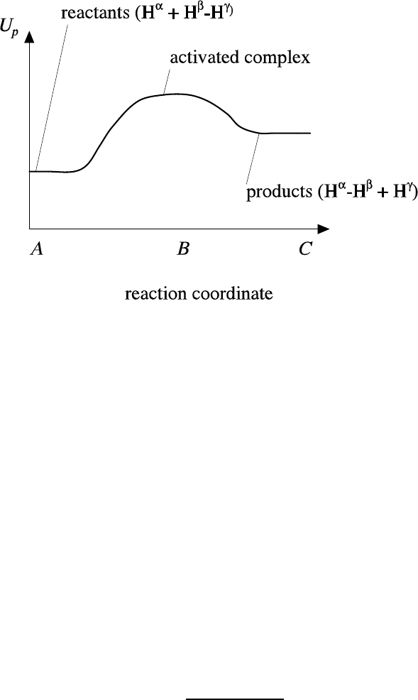
40
Fig. 2.4. Locus of local minima of the potential energy for the potential energy
contours shown in Fig. 2.3).
energies of the activated complex and the reactants. For the first of the
reactions (2.148)
E
0
≡ E
X
∗
− E
A
− E
BC
(2.150)
where E
X
∗
, E
A
and E
BC
are the zero point energies per mole of X
∗
, A, and
BC, respectively, relative to an arbitrary zero of energy.
For a one-dimensional vibration of a molecule, the partition function
is given by (McQuarrie, 2003, p. 96)
ˆq =
1
1 − e
−h ν/(k
b
T )
(2.151)

Review of background material 41
where ν is the frequency of vibration, h = 6.626 × 10
−34
J-s is Planck’s
constant, and k
b
= 1.38 ×10
−23
J/K is Boltzmann’s constant. It is assumed
that the activated complex crosses the saddle point via a very loose vibration,
i.e. the frequency ν → 0 (Laidler, 2007, p. 95). In this limit, (2.151) reduces
to
ˆq =
k
b
T
h ν
(2.152)
Thus
ˆq
X
∗
=
k
b
T
h ν
ˆq
0
X
∗
(2.153)
where ˆq
0
X
∗
represents the partition function for all the degrees of freedom of
the activated complex, except the loose vibration near the saddle point.
Equations (2.149) and (2.153) imply that
c
X
∗
=
N
a
k
b
T
h ν
(ˆq
0
X
∗
/V )
(ˆq
A
/V ) (ˆq
BC
/V )
e
−E
0
/(R T )
c
A
c
BC
(2.154)
As the time required for the activated complex to cross the saddle region is
≈ 1/ν, the molar reaction rate for the forward reaction is given by
˙
β =
c
X
∗
1/ν
=
R T
h
(ˆq
0
X
∗
/V )
(ˆq
A
/V ) (ˆq
BC
/V )
e
−E
0
/(R T )
c
A
c
BC
(2.155)
where R ≡ k
b
N
a
is the gas constant. Hence the rate constant for the forward
reaction is given by
k =
R T
h
(ˆq
0
X
∗
/V )
(ˆq
A
/V ) (ˆq
BC
/V )
e
−E
0
/(R T )
(2.156)
Note that the pre-exponential factor is now a function of the temperature,
unlike in the Arrhenius equation.
2.18.3 Comparison of the theories
For the reaction
A + B → AB (2.157)
where A and B are atoms, both the theories give identical expressions for the
rate constant (Laidler, 2007, pp. 106-107). For reactions involving molecules,
the partition functions occurring the activated complex theory involve other
degrees of freedom such as rotation and vibration in addition to transla-
tion, whereas the collision theory considers only translation. As discussed
in Laidler (2007, pp. 107-109), these additional degrees of freedom cause the
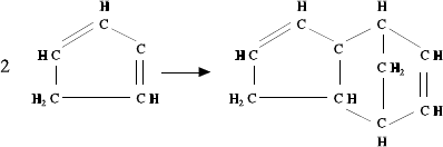
42
pre-exponential factor predicted the activated complex theory to be signifi-
cantly lower than than that predicted by the collision theory. Two examples
are given below.
Table 2.1 compares the measured and predicted pre-exponential fac-
tors for the dimerization of cyclopentadiene (Fig. 2.5)
2 C
5
H
6
(cyclopentadiene) → C
10
H
12
(2.158)
and
Fig. 2.5. Dimerization of cyclopentadiene.
2NO
2
→ 2 NO + O
2
(2.159)
In both the cases, the activated complex theory gives reasonable estimates
of the pre-exponential factors, whereas the collision theory overestimates
them considerably.
2.18.4 Reactions in solution
Some reactions occur in both the gas phase and also in a liquid solvent.
In such cases, the rate in solution is comparable to that in the gas phase
(Table 2.2), except for the dimerization reaction in C
6
H
6
. For reactions that

Review of background material 43
Table 2.1. Measured and predicted values of the pre-exponential factor A
for the reactions (2.158) and (2.159). Source: Laidler (1965, pp. 124-125).
A (m
3
/mol-s)
reaction (2.158) (2.159)
experiment 10
4
2 × 10
6
collision theory 10
8
4 × 10
7
activated complex theory 2 × 10
4
2.5 × 10
6
occur in solution, but not in the gas phase, the solvent may significantly
affect the rate (Table 2.3).
2.18.5 Catalytic reactions
A catalyst is a substance that increases the reaction rate without being
permanently affected by the reaction. As it increases the rates of the forward
and backward reactions by the same amount, the equilibrium conversion is
unaffected.
As noted by Laidler (2007, p. 229), the word catalysis is derived
from the Greek words kata (wholly) and lyein (loosen). The word catalyst
was coined by Berzelius (1836), who studied several reactions, and is usually
credited with the discovery of catalysis. However, as noted by Laidler and
Cornish-Bowden (1979) (cited in Datta, 2005, p. 248-249), the phenomenon
of catalysis had been discovered forty years earlier by Elizabeth Fulhame.
Catalytic reactions may be broadly classified as homogeneous or het-
erogeneous. In the former, the reactants, products, and catalyst are all in
the same phase; in the latter, more than one phase is involved. Enzyme
catalysis is usually classified under homogeneous catalysis (Laidler, 2007,
p. 378).
An example of a homogeneously catalyzed gas phase reaction is pro-
vided by the decomposition of acetaldehyde in the presence of iodine (Lai-
dler, 2007, p. 414):
CH
3
CHO → CH
4
+ CO (2.160)
Here I
2
acts as a catalyst, reducing the activation energy from about 200

44
Table 2.2. Comparison of pre-exponential factors A and activation energies
E for reactions in the gas phase and in liquids. Source: Laidler (2007,
pp. 184-185).
solvent log
10
A E
(A in m
3
/mol-s) (kJ/mol)
(i) decomposition of N
2
O
5
gas phase 7.6 103.3
CCl
4
7.6-7.8 101.3-106.7
CHCl
3
7.6-7.7 102.5-102.9
(ii) dimerization of cyclopentadiene
gas phase 0.1 69.9
CCl
4
-0.1 67.8
C
6
H
6
1.1 29.7
CS
2
-0.3 74.1
kJ/mol to about 135 kJ/mol. There are many aqueous phase reactions that
are catalyzed by acids and bases, such as the reaction between acetone and
iodine (Laidler, 2007, p. 392).
Many industrial reactions such as the synthesis of NH
3
involve het-
erogeneous (solid) catalysts. Such reactions involve several steps, such as
the mass transfer between the bulk fluid and the surface of the catalyst,
adsorption of reactants on the surface, either surface reactions between ad-
sorbed reactants or reactions between adsorbed and fluid-phase reactants,
and desorption of reactants and products from the surface.
In the context of the transition state theory, the main effect of a solid
catalyst is to lower the energy barrier (Fig. 2.6). For example, the activation
energy for the decomposition of NH
3
decreases from 340 kJ/mol to 134-180
kJ/mol when a molybdenum catalyst is used (Laidler, 2007, p. 267).
Consider the unimolecular reaction A
1
(g) → A
2
(g) which is cat-

Review of background material 45
Table 2.3. Effect on the solvent on the rate of reaction between
triethylamine and ethyliodide. Here k is the second order rate constant,
evaluated as 100
◦
. Source: Laidler (2007, p. 185).
solvent 10
11
k
(A in m
3
/mol-s)
hexane 0.5
toluene 25.3
benzene 39.8
alyzed by a solid catalyst. Suppose it is assumed that the surface reaction
is the rate-limiting step, i.e. of adsorption and desorption can occur at rates
that are potentially much faster than the rate of surface reaction. Hence
these processes may be assumed to be at equilibrium, and the concentrations
of the adsorbed species may be calculated using the adsorption isotherms.
The latter are obtained by equating the rates of adsorption and desorption
of each reactant, in the absence of reactions. The above model leads to the
rate expression (Schmidt, 2005, p. 303)
˙
β =
k K
1
p
1
1 + K
1
p
1
+ K
2
p
2
(2.161)
where
˙
β is the intrinsic reaction rate, k is the rate constant, K
i
and p
i
are
the adsorption equilibrium constants and partial pressure, respectively, of
species A
i
. Equation (2.163) assumes that A
2
is first formed as an adsorbed
species that then desorbs, i.e. the reactions involved are
A
1∗
→ A
2∗
→ A
2
g (2.162)
where A
1∗
represents adsorbed A
1
. If A
2
(g) is formed directly from A
1∗
, we
set K
2
= 0 in (2.163). Equation (2.163) represents an example of Lanmuir-
Hinshelwood, or equivalently, Hougen-Watson kinetics, named after Lang-
muir (1922), Hinshelwood (1926), and Hougen and Watson (1947) (cited in
Froment and Bischoff, 1990, p. 71). Instead of assuming that the surface
reaction is rate-limiting, alternative assumptions may be used, leading to
different rate expressions (Froment and Bischoff, 1990, pp. 76-77).

46
Similarly, for the reaction A
1
(g) + A
2
(g) → A
3
(g), the reaction
rate is given by (Schmidt, 2005, p. 308)
˙
β =
k K
1
K
2
p
1
p
2
(1 + K
1
p
1
+ K
2
p
2
+ K
3
p
3
)
2
(2.163)
As noted by Schmidt (2005, p. 309), the use of Langmuir-Hinshelwood kinet-
ics involves several assumptions that may not be justified in actual surface
catalyzed reactions. However, it provides relatively simple kinetic models
for complex heterogeneous catalytic reactions. Zhang et al. (2009) discuss
the use of such models for the Fischer-Tropsch synthesis of hydrocarbons
from water gas, which is a mixture of CO and H
2
.
2.18.6 Ideal reactors
As mentioned in Chapter 1, ideal reactors are based on simple models of
flow patterns and mixing in the reaction vessel.
(a) The ideal batch reactor
In an ideal batch reactor, the concentration and temperature fields
are assumed to be spatially uniform. In practice, the condition can be ap-
proximately realized by vigorous agitation or stirring. In the absence of
stirring, beautiful spatial patterns, caused by an interaction between dif-
fusion and reactions, may develop in some systems (Epstein et al., 1983;
Epstein and Showalter, 1996).
All the elements of the fluid spend the same amount of time in the
reactor, and hence have the same residence time. From the viewpoint of
thermodynamics, a batch reactor represents a closed system. The steady
states of the batch reactor correspond to states of reaction equilibria, which
satisfy (2.84).
Batch reactors are often used in the pharmaceutical industry, where
small volumes of high-value products are made.
(b) The ideal continuous stirred tank reactor (CSTR)
Like in an ideal batch reactor, the concentration and temperature
fields in an ideal CSTR are spatially uniform. As there are no spatial gra-
dients, the species concentrations in the exit stream are identical to the
corresponding values in the reactor. On the other hand, the species con-
centrations in the inlet stream are in general different from those in the
reactor.
Unlike the batch reactor, the CSTR is an open system as it can
Review of background material 47
exchange heat and mass with the surroundings. Hence it operates away from
equilibrium, and steady states are usually not states of reaction equilibria.
On account of the assumption of perfect mixing, the sequence in
which fluid elements leave the reactor is uncorrelated with the sequence in
which they enter. As shown later, this leads to a distribution of residence
times for the fluid leaving the reactor.
These reactors are widely used for polymerization reactions such as
the polymerization of styrene, production of explosives, synthetic rubber,
etc. Compared to tubular reactors, CSTRs are easier to clean and permit
better control of the temperature.
(c) The plug flow reactor (PFR)
The PFR is an idealization of a tubular reactor. The velocity, tem-
perature, and concentration fields are assumed to be uniform across the
cross section of the reactor. In practice, this situation can be approximately
realized for the case of turbulent flow through a tube with a large ratio of
the length to the diameter. The latter condition ensures that axial mixing
has a negligible effect on the conversion.
In a PFR, there is perfect mixing in the radial or transverse direction.
Further, there is no mixing or diffusion in the axial direction. Like a CSTR,
the PFR also represents an open system, and hence steady states are not
states of reaction equilibrium. Owing to the assumption of plug flow, all
the fluid elements have the same residence time. The velocity of the fluid is
often treated as a constant, but this assumption must be relaxed when the
density of the fluid changes significantly along the length of the tube.
The steady state equations for a PFR are similar in form to the
dynamic equations for an ideal batch reactor. In many cases, the results
for the latter can be translated into results for a PFR operating at a steady
state.
Tubular reactors are used for many gas phase and liquid phase reac-
tions, such as the oxidation of NO and the synthesis of NH
3
. These reactors
are often modelled as PFRs, but more detailed models involving complica-
tions such as radial gradients, may be required in some cases.

48
Fig. 2.6. Variation of the potential energy U
p
along the reaction coordinate for an
uncatalyzed gas phase reaction (—) and a solid catalyzed heterogeneous reaction
(- - -). Here A, C, D, and G denote the gaseous reactants, gaseous products,
adsorbed reactants, and adsorbed products, respectively. and D and F denote the
activated complexes for the gas phase and heterogeneous reactions, respectively.
The quantities ∆U
ph
and ∆U
pc
represent the energy barriers for the homogeneous
and catalytic reactions, respectively. Adapted from Laidler (2007, p. 268).
References
Agar, D. W. (1999). Multifunctional reactors: old preconceptions and new
dimensions. Chem. Engng Sci. 54, 1299–1305.
Altinten, A., Ketavanlioglu, F., Erdogan, S., Hapoglu, H., and Alpbaz, M.
(2008). Self-tuning PID control of jacketed batch polystyrene reactor using
genetic algorithm. Chem. Engg. J. 138, 490–497.
Aneshansley, D. J., Eisner, T., Widom, J. M., and Widom, B. (1969). Bio-
chemistry at 100
◦
C: Explosive secretory discharge of bombardier beetles
(brachinus). Science 165, 61–63.
Arfken, G, B. and Weber, H. J. (2001). Mathematical Methods for Physicists,
5 edn. (Academic Press, San Diego).
Aris, R. (1999). Elementary Chemical Reactor Analysis. (Dover, Mineola).
Arrhenius, S. (1899). Uber die reaktionsgeschwindigkeit bei der inversion
von rohrzucker dur sauren (On the reaction velocity of the inversion of
cane sugar by acids). Z. Phys. Chem. 4, 226.
Atkins, P. W. and de Paula, J. (2002). Physical Chemistry, 7 edn. (Oxford
University Press, Oxford).
Berzelius, J. (1836). Jahres-bericht uber die forschritte der physichen wis-
senschaft. Tech. rep., Tubingen.
Blum, E. H. and Luus, R. (1964). Thermodynamic consistency of reaction
rate expressions. Chem. Eng. Sci. 19, 322–323.
Bodenstein, M. and Lind, S. C. (1907). Z. Phys. Chem. 57, 108.
Callen, H. B. (1985). Thermodynamics, 2 edn. (Wiley, New York).
Chatterjee, I. B. and Joshi, J. B. (2008). Modelling, simulation, and op-
timization: Mono pressure nitric acid process. Chem. Engng J. 138,
556–577.
Christiansen, J. A. (1919). K. Dan. Vidensk. Selsk. Mat.-Fys. Medd. 1, 14.
49
50 REFERENCES
Datta, N. C. (2005). The Story of Chemistry. (Univerisities Press, Hyder-
abad).
de Donder, T. (1922). Bull. Acad. Belg. Cl. Sci. 8, 197.
Denbigh, K. G. (1971). The Principles of Chemical Equilibrium, 3 edn.
(Cambridge University Press, Cambridge).
Denbigh, K. G. and Turner, J. C. R. (1972). Chemical Reactor Theory,
2 edn. (The Engligh Language Book Society and Cambridge University
Press, Cambridge).
Dodge, B. F. (1944). Chemical Engineering Thermodynamics. (McGraw-
Hill, New York).
Epstein, I. R., Kustin, K., De Kepper, P., and Orban, M. (1983). Oscillating
chemical reactions. Sci. Am. 248, 96–108, 130.
Epstein, I. R. and Showalter, K. (1996). Nonlinear chemical dynamics:
oscillations, patterns, chaos. J. Phys. Chem. 100, 13132–13147.
Evans, M. G. and Polanyi, M. (1935). Some applications of the transition
state method to the calculation of reaction velocities, especially in solu-
tion. Trans. Faraday Soc. 31, 875–894.
Eyring, H. (1935). The activated complex in chemical reactions. J. Chem.
Phys. 3, 107–115.
Fan, X., Manchon, M. G., Wilson, K., Tennison, S., Kozynchenko, A., Lap-
kin, a., and Pluchinski, P. K. (2009). Coupling of Heck and hydrogenation
reactions in a continuous compact reactor. J. Cat. 267, 114–120.
Fogler, H. S. (1999). Elements of Chemical Reaction Engineering, 3 edn.
(Prentice-Hall of India, New Delhi).
Froment, G. F. and Bischoff, K. B. (1990). Chemical Reactor Analysis and
Design, 2 edn. (Wiley, New York).
Frost, A. A. and Pearson, R. G. (1961). Kinetics and Mechanism, 2 edn.
(Wiley-Toppan, Tokyo).
Gerald, C. F. and Wheatley, P. O. (1994). Applied Numerical Analysis, 5
edn. (Addison-Wesley, Reading).
Gillou, L., Paul, S., and Le Courtois, V. (2008). Investigation of H
2
staging
effects on CO conversion and product distribution for Fischer-Tropsch
synthesis in a structured microchannel reactor. Chem. Engng. Sci. 136,
66–76.
Guldberg, C. M. and Waage, P. (1864). Forh. Vid. Selsk. Christiania 35,
111.
Harcourt, A. V. and Esson, W. (1895). On the laws of connexion between the
conditions of a chemical change and its amount. III. Further research on
the reaction between hydrogen dioxide and hydrogen iodide. Phil. Trans.
Roy. Soc. London A 186, 817–895.
REFERENCES 51
Heintz, A., Kapteina, S., and Verevkin, S. P. (2007). Comprehensive experi-
mental and theoretical study of chemical equilibria in the reacting system
of the t-amyl methyl ether synthesis. J. Phys. Chem. B 111, 10975–10984.
Henri, V. (1902). Th´eorie g´eneral´e de l’action de quelques diastates. C. R.
Hebd. Seanc. Acad. Sci. Paris 135, 916–919.
Herzfeld, K. F. (1919). Z. Elektrochem. 25, 301.
Hinshelwood, C. N. (1926). Kinetics of Chemical Change in Gaseous Sys-
tems. (Clarendon Press, Oxford).
Hougen, O. A. and Watson, K. M. (1947). Chemical Process Principles, Vol.
III. (Wiley, New York).
Jackson, R. (2000). The Dynamics of Fluidized Particles. (Cambridge Uni-
versity Press, Cambridge).
Kooij, D. M. (1893). Z. Phys. Chem. 12, 155.
Kooijman, S. A. L. M. (2001). Quantitative aspects of metabolic organi-
zation: a discussion of concepts. Phil. Trans. Roy. Soc. Lond. B 56,
331–349.
Kreyszig, E. (1993). Advanced Engineering Mathematics, 7 edn. (Wiley,
New York).
Laidler, K. J. (1965). Chemical Kinetics. (McGraw-Hill, New York).
Laidler, K. J. (2007). Chemical Kinetics, 3 edn. (Pearson Education, New
Delhi).
Laidler, K. J. and Cornish-Bowden, A. (1979). Elizabeth fulhame and the
discovery of catalysis - 100 years before buchner. In New Beer in an
Old Bottle: Eduard Buchner and the Growth of Biochemical Knowledge,
A. Cornish-Bowden, ed. (Universitat de Valencia, Spain).
Langmuir, I. (1922). The mechanism of the catalytic action of platinum in
the reactions 2 CO + O
2
= 2 CO
2
and 2 H
2
+ O
2
= 2 H
2
O. Trans.
Faraday Soc. 17, 621–654.
Lee, W. J. and Li, C.-Z. (2009). Catalytic reactions of hydrogen in a fluidized
be reactor with Ni nanoparticles. Energy and Fuels 23, 4866–4870.
Levenspiel, O. (2004). Chemical Reaction Engineering, 3 edn. (Wiley India,
New Delhi).
Lewis, W. M. M. (1918). J. Chem. Soc. (London) 113, 471.
McQuarrie, D. A. (2003). Statistical Mechanics. (Viva Books, New Delhi).
Michaelis, L. and Menten, M. L. (1913). Die kinetic der invertinwirkung.
Biochem. Z. 49, 333–369.
Morrison, R. T. and Boyd, R. N. (2002). Organic Chemistry, 6 edn. (Pearson
Education, New Delhi).
Pelzer, H. and Wigner, E. (1932). Uber die geschwindigkeitskonstante von
auystanuschreaktionen. Z. Phys. Chem. B 15, 445–463.
52 REFERENCES
Pereira, C. J. (1999). Environmentally friendly processes. Chem. Engng.
Sci. 54, 1959–1973.
Polanyi, M. (1920). Z. Electrochem. 26, 50.
Prausnitz, J. M., Lichtenthaler, R. N., and de Azevedo, E. G. (1999). Molec-
ular Thermodynamics of Fluid-Phase Equilibria, 3 edn. (Prentice-Hall,
Upper Sadle River).
Rahimpour, M. R. and Ghader, S. (2004). Enhancement of CO conversion
in a novel Pd-Ag membrane reactor for methanol synthesis. Chem. Eng.
Proc. 43, 1181–1188.
Sandler, S. I. (2006). Chemical, Biochemical, and Engineering Thermody-
namics, 4 edn. (Wiley India, New Delhi).
Sawyer, C. N., McCarty, P. L., and Parkin, G. F. (2003). Chemistry for
Environmental Engineering and Science, 5 edn. (Tata McGraw-Hill, New
Delhi).
Schmidt, L. D. (2005). The Engineering of Chemical Reactions, 2 edn.
(Oxford, New York).
Shuler, M. L. and Kargi, F. (2004). Bioprocess Engineering, 2 edn. (Prentice-
Hall of India, New Delhi).
Smith, J. M., Van Ness, H. C., and Abbott, M. M. (2001). Introduction
to Chemical Engineering Thermodynamics, 6 edn. (McGraw-Hill, New
York).
Sotowa, K.-I., Shirashi, N., Iguchi, Y., and Sugiyama, S. (2008). Forced
temperature cycling of a catalyst layer and its application to propylene
oxidation. Chem. Engng Sci. 63, 2690–2695.
Sundaram, K. M. and Froment, G. F. (1977). Modeling thermal cracking
kinetics - I. Chem. Eng. Sci. 32, 601–608.
Tokumura, M., Katoh, T., Ohata, H., and Kawase, Y. (2009). Dynamic
modelling and simulation of ozonation in a semibatch bubble column re-
actor: decolorization and mineralization of azo dye orange II by ozone.
Ind. Eng. Chem. Res. 48, 7965–7975.
Trautz, M. (1916). Das gesetz der reaktionsgeschwindigkeit und der gle-
ichguwechte in gasen. bestatigung der additivitat von c
v
− 3/2R. neue
bestimmung der integrationskonstanten und der molekuldurchmesses. Z.
Anorganische unn Allgemeine Chemie 96, 1–28.
Truhlar, D. G. and Horowitz, C. J. (1978). Functional representation of Liu
and Siegbahn’s accurate ab initio potential energy calculations for H +
H
2
. J. Chem. Phys. 68, 2466–2476.
van’t Hoff, J. H. (1884). Etudes de dynamique chimique. (Muller, Amster-
dam).
REFERENCES 53
Wang, N., Matsumoto, T., Ueno, M., Miyamura, H., and Kobayashi, S.
(2009). A gold-immobilized microchannel reactor for oxidation of alcohols
with moelcular O
2
. Angew. Chem. Intl. Ed. 48, 4744–4746.
Wu, Q., Hu, X., Yue, P. L., Feng, J., Chen, X., Zhang, H., and Qiao,
S. (2009). Modeling of a pilot-scale trickle bed reactor for the catalytic
oxidation of phenol. Sep. Purif. Tech. 67, 158–165.
Wynne-Jones, W. F. K. and Eyring, H. (1935). The absolute rate of reactions
in condensed phases. J. Chem. Phys. 3, 492–502.
Yang, B., Zhou, X.-W., Yang, X.-H., Chen, C., and Wang, L.-Y. (2009).
Multi-scale study on the secondary reaction of fluid catalytic cracking
gasoline. AIChE J. 55, 2138–2149.
Yu, L., Lu, J., Zhang, X., and Zhang, S. (2007). Numerical simulation of the
bubbling fluidized bed coal gasification by the kinetic theory of granular
flow. Fuel 86, 722–734.
Zhang, R., Chang, J., Xu, Y., Cao, L., Li, Y., and Zhou, J. (2009). Ki-
netic model of product distribution over Fe catalyst for Fischer-Tropsch
synthesis. Energy Fuels 23, 4740–4747.
