Pre-K–12 Guidelines for Assessment and Instruction in Statistics

Pre-K–12 Guidelines for Assessment and Instruction

in Statistics Education II (GAISE II)

A Framework for Statistics and Data Science Education

Writing Committee

Anna Bargagliotti (co-chair)

Loyola Marymount University

Christine Franklin (co-chair)

American Statistical Association

Pip Arnold

Karekare Education New Zealand

Sheri Johnson

University of Georgia*

Leticia Perez

University of California Los Angeles Center X

Denise A. Spangler

University of Georgia

Rob Gould

University of California Los Angeles

The Pre-K–12 Guidelines for Assessment and Instruction in Statistics Education II (GAISE II)

is an official position of the National Council of Teachers of Mathematics as approved by the

NCTM Board of Directors, February 2020.

Endorsed by the American Statistical Association, November 2020.

*Current affiliation -The Mount Vernon School

Library of Congress Cataloging-in-Publication Data

Names: Bargagliotti, Anna, author.

Title: Pre-K–12 guidelines for assessment and instruction in statistics

education II (GAISE II) / writing committee, Anna Bargagliotti

(co-chair), Loyola Marymount University, Christine Franklin (co-chair),

American Statistical Association, Pip Arnold, Karekare Education New

Zealand, Rob Gould, University of California Los Angeles, Sheri Johnson,

University of Georgia, Leticia Perez, University of California Los

Angeles, Denise A. Spangler, University of Georgia.

Other titles: Guidelines for assessment and instruction in statistics

education (GAISE) report

Description: Second edition. | Alexandria, VA : American Statistical

Association, 2020. | Includes bibliographical references. | Summary:

“This document lays out a curriculum framework for Pre-K–12 educational

programs that is designed to help students achieve data literacy and

become statistically literate. The framework and subsequent sections in

this book recommend curriculum and implementation strategies covering

Pre-K–12 statistics education”-- Provided by publisher.

Identiﬁers: LCCN 2020006082 | ISBN 9781734223514 (paperback)

Subjects: LCSH: Statistics--Study and teaching (Early

childhood)--Standards. | Statistics--Study and teaching

(Elementary)--Standards. | Statistics--Study and teaching

(Secondary)--Standards.

Classiﬁcation: LCC QA276.18 .G85 2020 | DDC 519.5071/2--dc23

LC record available at https://lccn.loc.gov/2020006082

Alexandria, VA 22314

Printed in the United States of America

10 9 8 7 6 5 4 3 2 1

978-1-7342235-1-4

Contents

Acknowledgments ............................................................................................................................v

Preface ................................................................................................................................................1

Introduction ........................................................................................................................................5

Framework ........................................................................................................................................13

Level A ...............................................................................................................................................21

Introduction ............................................................................................................................................ 22

Essentials for Each Component ............................................................................................................ 22

Example 1: Choosing the Band for the End of the Year Party –

Conducting a Survey and Summarizing Data ........................................................................ 24

Example 2: Family Size - Mean as Equal/Fair Share and Variability as Number of Steps .......................... 28

Example 3: What do Ladybugs Look Like – Collecting, Summarizing, and Comparing Data .................... 31

Example 4: Growing Beans – A Simple Comparative Experiment ............................................................ 35

Example 5: Growing Beans (Continued) – Time Series ............................................................................ 37

Example 6: CensusAtSchool – Using Secondary Data and Looking at Association .................................. 38

Summary of Level A ............................................................................................................................... 41

Level B ...............................................................................................................................................43

Introduction ............................................................................................................................................ 44

Essentials for Each Component ............................................................................................................ 44

Example 1: Level A Revisited: Choosing the Music for the School Dance –

Multivariable and Larger Groups ............................................................................................ 45

Example 2: Choosing Music for the School Dance (Continued) – Comparing Groups .............................. 49

Example 3: Choosing Music for the School Dance (Continued) –

Connecting Two Categorical Variables ................................................................................... 51

Example 4: Darwin’s Finches – Comparing a Quantitative Variable Across Groups ................................... 53

Example 5: Darwin’s Finches (Continued) – Separation Versus Overlap ................................................... 57

Example 6: Darwin’s Finches (Continued) – Measuring the Strength of Association

Between Two Quantitative Variables ...................................................................................... 59

Example 7: Darwin’s Finches (Continued) – Time Series .......................................................................... 61

Example 8: Dollar Street – Pictures as Data ............................................................................................. 62

Example 9: Memory and Music – Comparative Experiment ..................................................................... 67

Summary of Level B ............................................................................................................................... 68

| iii

Pre-K–12 Guidelines for Assessment and Instruction in Statistics Education II (GAISE II)

iv |

Level C ............................................................................................................................................... 71

Introduction ............................................................................................................................................ 72

The Role of Technology ......................................................................................................................... 73

The Role of Probability in Statistics Essentials for Each Component ................................................. 73

Example 1: Darwin’s Finches from Level B (Continued) – MAD to Standard Deviation .............................. 77

Example 2: Level A and B Revisited: Choosing Music for the School Dance – Generalizing Findings ....... 79

Example 3: Choosing Music for the School Dance (Continued) – Inference About Association ................. 83

Example 4: Effects of Light on the Growth of Radish Seedlings – Experiments ........................................ 84

Example 5: Considering Measurements When Designing Clothing – Linear Regression ........................... 89

Example 6: Napping and Heart Attacks – Inferring Association from an Observational Study ................... 92

Example 7: Working-age Population – Working with Secondary Data ...................................................... 94

Example 8: Classifying Lizards – Predicting a Categorical Variable ........................................................... 97

Summary of Level C ............................................................................................................................. 102

Assessment ....................................................................................................................................105

National and International Standardized Assessments ..................................................................... 105

Sources of Quality Items for Educators .............................................................................................. 105

Level A Assessment Examples ............................................................................................................ 106

Level B Assessment Examples ........................................................................................................... 108

Level C Assessment Examples ........................................................................................................... 111

References ......................................................................................................................................115

| v

GAISE II Acknowledgements

A special thank you to Christine Franklin, Gary Kader, Denise Mewborn (Spangler) Jerry Moreno,

Roxy Peck, Mike Perry, and Richard Scheaffer for their leadership and vision in the first seminal

GAISE I document.

The authors extend a sincere thank you to the ASA/NCTM Joint Committee for funding the writing

and production process of GAISE II. A special thank you to Donna LaLonde and Rebecca Nichols

from ASA and Dave Barnes and Jeff Shih from NCTM for their support throughout the process.

Thank you to Brenna Bastian for her beautiful artwork on the cover of the report and the Level A Ladybugs

Example. We also appreciate the design and layout work of Shirley E.M. Raybuck and Valerie Nirala.

Lastly, the authors would like to express their heartfelt appreciation to the twenty-two people who

closely reviewed this GAISE II document and provided valuable feedback:

Gail Burrill, Rosemarie Callingham, Catherine Case , Michelle Dalrymple, Neville Davies, Ed Dickey,

David Fluharty, Gary Kader, Donna LaLonde, Jerry Moreno, Rebecca Nichols, Regina Nuzzo,

Roxy Peck, Jamis Perrett , Maxine Pfannkuch, Katherine Respress, Richard Schaeffer, Neil Sheldon,

Josh Tabor, Dan Teague, Doug Tyson, and Jane Watson.

| 1

GAISE II Preface

In 2020 as the Pre-K–12 Guidelines for Assessment and Instruction in Statistics Education II: A Framework for

Statistics and Data Science Education report (GAISE II) is published, never have data and statistical literacy

been more important. The public is being called upon to synthesize information from many global issues,

including the COVID-19 global pandemic, a changing planet with extreme weather conditions, economic

upturns and downturns, and important social issues such as the Black Lives Matter movement. Data are

encountered through visualizations (sometimes interactive and sometimes not), reports from scientific

studies (such as medical studies), journalists’ articles and websites.

The demands for statistical literacy have never been greater. Statistically literate high-school graduate need

to be able to evaluate the conclusions and legitimacy of reported results as well as formulate their own

analyses. Steve Levitt, co-author of Freakonomics, addressed the need for statistical and data literacy with

this quote from an October 2, 2019 podcast:

I believe that we owe it to our children to prepare them for the world that they will encounter—a world

driven by data. Basic data fluency is a requirement not just for most good jobs, but also for navigating

life more generally, whether it is in terms of financial literacy, making good choices about our own

health, or knowing who and what to believe.

Driven by the digital revolution, data are now readily accessible to statistical methods and technological

tools so that students can gain insights and make recommendations to manage pressing world issues. Data

can be extremely valuable, but only if they are used judiciously and in a proper context.

Today, many sectors of the economy and most jobs rely on data skills. Good data sense is needed to easily

read the news and to participate in society as a well-informed member. Because of this, it is essential that all

students leave secondary school prepared to live and work in a data-driven world. The Pre-K–12 GAISE II

report presents a set of recommendations for school-level statistical literacy.

Overview and Goals of GAISE II

Guidelines for Assessment and Instruction in Statistics Education: A Pre-K–12 Curriculum Framework

(hereafter referred to as Pre-K–12 GAISE I) was first released in 2005 with slight revisions in 2007 (https://

www.amstat.org/asa/files/pdfs/GAISE/GAISEPreK-12_Full.pdf) along with the Guidelines for Assessment

and Instruction in Statistics Education College Report. The GAISE College Report outlined recommendations

for the post-secondary introductory statistics course and was updated in 2016 (https://www.amstat.org/

asa/files/pdfs/GAISE/GaiseCollege_Full.pdf).

The Pre-K–12 GAISE I report was written to enhance the statistics standards in the National Council for

Teachers of Mathematics (NCTM) 2000 Principles and Standards of School Mathematics and as a follow-up

document to the Conference Board of Mathematical Sciences (CBMS) Mathematical Education for Teachers

(MET) document. The Pre-K–12 GAISE I was a seminal and visionary document that championed the

necessity of data and statistical literacy starting in the early school grades. It provided a framework of

recommendations for developing students’ foundational skills in statistical reasoning in three levels across

Pre-K–12 Guidelines for Assessment and Instruction in Statistics Education II (GAISE II)

2 |

the school years, described as levels A, B, and C. These levels are maintained in GAISE II and are roughly

equivalent to elementary, middle, and high school. The progression through the sequential levels in the

Pre-K–12 GAISE (both I and II) is intended for any individual who is striving to achieve statistical

literacy, regardless of age.

Since its initial publication, GAISE I has significantly impacted the inclusion of statistics standards at the

state and national level in the United States and across the world. The report has been used internationally

as a reference point for statistics education at the school level. There is a Spanish translation of GAISE I

(https://www.amstat.org/asa/files/pdfs/GAISE/Spanish.pdf). At the time of this writing, Google scholar

shows over 790 citations for GAISE I in scholarly works. The report has been referenced in numerous

National Science Foundation grant projects and other professional STEM educational organizations’

reports. GAISE I also influenced the development of state standards across the United States and the

writing of the ASA Statistical Education of Teachers (SET) document (https://www.amstat.org/asa/

files/pdfs/EDU-SET.pdf ) that makes recommendations for the preparation of school level teachers in

statistics.

GAISE I primarily focused on traditional data types of quantitative and categorical variables and on

study designs using small data sets of samples from a population. Fifteen years later, data types have

expanded beyond being classified as quantitative and categorical thus necessitating the acquisition of

different and often state-of-the-art statistical skills. Today, for example, data include text posted on social

media or highly structured (or unstructured) collections of pictures, sounds, or videos. Data are immense

and readily available. Data are multidimensional. Data representations and visualizations are also often

multidimensional and interactive displaying many variables simultaneously.

GAISE II incorporates the new skills needed for making sense of data today while maintaining the spirit

of GAISE I. GAISE II highlights:

1. The importance of asking questions throughout the statistical problem-solving process (for-

mulating a statistical investigative question, collecting or considering data, analyzing data, and

interpreting results), and how this process remains at the forefront of statistical reasoning for

all studies involving data

2. The consideration of different data and variable types, the importance of carefully planning

how to collect data or how to consider data to help answer statistical investigative questions,

and the process of collecting, cleaning, interrogating, and analyzing the data

3. The inclusion of multivariate thinking throughout all Pre-K–12 educational levels

4. The role of probabilistic thinking in quantifying randomness throughout all levels

5. The recognition that modern statistical practice is intertwined with technology, and the im-

portance of incorporating technology as feasible

6. The enhanced importance of clearly and accurately communicating statistical information

7. The role of assessment at the school level, especially items that measure conceptual under-

standing and require statistical reasoning involving the statistical problem-solving process

| 3

Preface

A Future Driven by Data

As stated in GAISE II,

Data are used to tell a story. Statisticians see the world through data – data serve as models of reality.

Statistical thinking and the statistical problem-solving process are foundational to exploring all data.

GAISE II presents a vision where every individual is confident in reasoning statistically, making sense

of data, and knowing how and when to bring a healthy skepticism to information gleaned from data.

Presented here is a framework of essential concepts and 22 examples across the three levels of skills

development. This framework supports all students as they learn to appreciate the vital role of statistical

reasoning and data science and acquire the essential life skill of data literacy.

We, the writers, are appreciative of the opportunity, support, and endorsement from the Board of

Directors of both the American Statistical Association (ASA) and the National Council for the Teachers

of Mathematics (NCTM) for the enhancement of the Pre-K–12 GAISE I document. Our hope is that

the Pre-K–12 GAISE II document will enrich your work in fostering the ultimate goal: statistical literacy

for all.

Anna Bargagliotti (co-chair)

Christine Franklin (co-chair)

Pip Arnold

Rob Gould

Sheri Johnson

Leticia Perez

Denise A. Spangler

| 5

Introduction

Our lives are heavily influenced by data. Every person should be able to use sound statistical reasoning to

intelligently make evidence-based decisions. We need statistical literacy to succeed at work, stay informed

about current events, and be prepared for a healthy, happy, and productive life.

Each morning, the newspaper and other media confront us with statistical information on topics ranging

from the economy to education, from movies to sports, from food to medicine, and from public opinion

to social behavior. Such information guides decisions in our personal lives and enables us to meet our

responsibilities as members of a community and society. Statistical literacy is a requirement for navigating

today’s world.

Data can also provide support in our personal lives. Wearing a fitness device allows us to track steps,

heart rate, and other fitness statistics in a way that motivates healthier lifestyles. If we consider moving to

another community, we could make decisions based on statistics about the cost of living or local climate.

Statistically literate individuals may have the opportunity to advance in their careers and obtain more

rewarding and challenging positions. Business leaders may be presented with quantitative information on

budgets, supplies, manufacturing specifications, market demands, sales forecasts, or workloads. Teachers

may be confronted with educational statistics concerning student performance or their own accountability.

Medical scientists must understand the statistical results of experiments used for testing the effectiveness

and safety of medical treatments. Law enforcement professionals depend on crime statistics.

Statistical literacy involves having a healthy dose of skepticism about findings based upon data. A statistically

literate high school graduate will be able to evaluate conclusions from data and judge the legitimacy of

reported results. The Business Higher Education Forum (BHEF) report The New Foundational Skills of the

Digital Economy agrees and states (www.bhef.com/sites/default/files/BHEF_2018_New_Foundational_

Skills.pdf ):

At some moment in the future, many of the high levels of skill that currently seem confined to the upper

reaches of the digital economy, or to larger, more complex organizations, will become the norm among

jobseekers, incumbent employees, and workplaces. (BHEF 2018 publication, p. 18)

The ultimate goal: statistical literacy for all.

Sound statistical skills take time to develop. They cannot be honed to the level needed in the modern world

through one high school course. The best way to help people attain statistical literacy is to begin their

statistics education in the elementary grades and keep strengthening and expanding students’ statistical

skills throughout middle school and high school years.

This document lays out a curriculum framework for Pre-K–12 educational programs that is designed to help

students achieve data literacy and become statistically literate. The framework and the subsequent sections

in this report recommend curriculum and implementation strategies covering Pre-K–12 statistics education.

Pre-K–12 Guidelines for Assessment and Instruction in Statistics Education II (GAISE II)

6 |

While the document provides a Pre-K–12 education framework, the pathway to statistical literacy

presented in this document is appropriate for any age bracket. In fact, the document’s framework is

meant for any individuals working towards statistical literacy. Throughout the report these individuals are

referred to as simply “students.”

Why Guidelines for Assessment and Instruction in Statistics

Education (GAISE) II? Overview and Goals of GAISE II

The Guidelines for Assessment and Instruction in Statistics Education: A Pre-K–12 Curriculum

Framework (GAISE I) was first released in 2005 with a slight revision in 2007 (see Figure 1). This was

a groundbreaking document. It made the case for statistical literacy at the school-level and explained

how mathematical and statistical thinking are related yet distinct. Mathematical skills are necessary, and

statistical and mathematical thinking must work in concert when analyzing data.

Since GAISE I was published, traditional conceptions of data have changed. Data are no longer simply

numbers in context, classified as quantitative or categorical, typically stored in static spreadsheets. Today,

data can also be dynamic, complex, highly structured (or unstructured) collections of pictures or sounds.

Data sets are vast and readily available.

Figure 1: GAISE I was rst released in 2005.

GAISE II includes examples that deal with non-traditional data and multivariable data throughout the

entire Pre-K–12 curriculum. Students must develop statistical literacy to make sense of the immense

amount of data that surround them on a daily basis. Much of these data are generated by students

themselves through social media, global positioning system (GPS) devices, and so on. Students should

become aware of how these data are stored and how they are utilized by the organizations collecting

them. They should also understand why our society needs security measures and policies to prevent the

mishandling and unethical use of these data.

Introduction

| 7

Students need to begin at an early age to become data-savvy, whether working with small data sets or large,

messy data sets, with traditional data or non-traditional data such as text or images. Most future jobs will

require some knowledge of statistics and data analytics.

Being able to reason statistically is essential in all disciplines of study and work. Many disciplines such as

the sciences now include statistics in their standards (e.g., Next Generation Science Standards (NGSS) Lead

States, 2013). Several of the new examples in GAISE II use science data sets and touch on topics discussed

in the Next Generation Science Standards (NGSS) to illustrate how statistical reasoning is an integral

component of scientific investigations.

While progress has been made over the past 50 years in preparing students, there is still much work

necessary for the future as the discipline of statistics continues to evolve. Some important documents since

the publication of GAISE I promoting statistical literacy at the Pre-K–12 school-level are The American

Statistical Association (ASA)’s Statistical Education of Teachers (SET) published in 2015 and National

Council of Teachers of Mathematics (NCTM)’s Catalyzing Change: Initiating Critical Conversations books

for elementary, middle (2020), and high school (2018). Those interested in learning about the history of

statistics in the Pre-K–12 setting may refer to Chapter 9 in SET.

The spirit of the original GAISE I report remains. The statistical problem-solving process defined in

GAISE I remains the foundation and core of statistical reasoning and making sense of data. The statistical

problem-solving process is defined as a four-step process of (1) formulating a statistical investigative

question, (2) collecting or considering data, (3) analyzing data, and (4) interpreting results. The three

levels of A, B, and C (loosely meant to match elementary, middle, and high school) are also consistent

across the GAISE I and GAISE II reports.

Spurred by the overabundance of data available in today’s world, the statistical problem-solving process

not only remains important, it becomes even more critical for drawing conclusions from data. This

includes recognizing misleading graphical representations and limitations of data sets, no matter how

large, being used to answer statistical investigative questions. For examples of misuses in statistics and

limitations of data sets see the following: The New York Times Magazine’s When the Revolution Came for

Amy Cuddy (www.nytimes.com/2017/10/18/magazine/when-the-revolution-came-for-amy-cuddy.html)

and Kuiper’s Incorporating Research Experience into an Early Undergraduate Statistics Course (http://iase-

web.org/documents/papers/icots8/ICOTS8_4G1_KUIPER.pdf?1402524970).

Statistically sound studies should be reproducible. Repeated studies with similar samples should

yield similar conclusions, and different statistical methods re-applied to the same data should give

consistent results.

As emphasized in the original GAISE, “statistics is a methodological discipline. It exists not for itself, but

rather to offer other fields of study a coherent set of ideas and tools for dealing with data. The need for

such a discipline arises from the omnipresence of variability” (Cobb & Moore, 1997, p. 801). Statistical

thinking, in large part, must deal with the omnipresence of variability in data (e.g., variability within a

group, variability between groups, sample-to-sample variability in a statistic). Statistical problem solving

and decision making depend on understanding, explaining, and quantifying variability in the data within

the given context. “Statistics requires a different kind of thinking, because data are not just numbers,

they are numbers with a context” (Cobb & Moore, 1997, p. 801). “In mathematics, context obscures

structure. In data analysis, context provides meaning” (Ibid, p. 803).

Pre-K–12 Guidelines for Assessment and Instruction in Statistics Education II (GAISE II)

8 |

To highlight the importance of statistical literacy today, consider the following graph in Figure 2 from The

New York Times’s What’s Going On in This Graph? from April 9, 2018.

Figure 2: : Distributions of projected earnings for different professions.

Source: The New York Times’s What’s Going On in This Graph? April 9, 2018

“The Lifetime Earnings Premia of Different Majors,” 2014 (updated: 2017), by Douglas A. Webber

This graphic displays the distributions of projected earnings for different professions. The distributions

are represented with bars where the bars are divided into segments by the 10

, 25

, 50

, 75

, and 90

percentiles (measures of positions for each distribution). Both the context and variability of the different

distributions are important when interpreting this graphic. For example, we can notice that education is

one of the lower-paying professions compared to chemical engineering, but there is also more variability for

the salaries of chemical engineers (note the length of the segments within the bars). Context is important,

too. We notice that this graphical display provides little information about how the data were obtained.

It is important to question how the data were obtained – are they primary data collected by researchers or

are they secondary data made available to investigators?

It is these features—the focus on variability in data, the importance of context associated with the data,

and the questioning of data—that sets statistics apart from other mathematical sciences and makes it

particularly relevant for all fields of study.

It is critical that statisticians—or anyone who uses data—be more than just data crunchers. They

should be data problem solvers who interrogate the data and utilize questioning throughout the

statistical problem-solving process to make decisions with confidence, understanding that the art

of communication with data is essential.

This report, therefore, enhances and updates the GAISE I report of 2005 and 2007 to adjust for the

remarkable evolution within the statistical field over the past 15 years. These enhancements include an

emphasis on:

• Questioning throughout the statistical problem-solving process

• Different data and variable types

Introduction

| 9

• Multivariable thinking throughout Levels A, B, and C

• Probabilistic thinking throughout Levels A, B, and C

• The role of technology in statistics and how it develops throughout the Levels

• Assessment items that measure statistical reasoning

Questioning in Statistics

Regardless of the kind of data with which we’re working — whether small samples from a population,

experimental data . . . addressing each component of the process is essential.

The statistical problem-solving process typically starts with a statistical investigative question, followed by

a study designed to collect data that aligns with answering the question. Analysis of the data is also guided

by questioning. Constant questioning and interrogation of the data throughout the statistical problem-

solving process can lead to the posing of new statistical investigative questions.

Often when considering secondary data, the data need to first be interrogated – how were measurements

made, what type of data were selected, what is the meaning of the data, and what was the study design to

collect the data. Once a better understanding of the data has been gained, then one can judge whether the

data set is appropriate for exploring the original statistical investigative question or one can pose statistical

investigative questions that can be explored with the secondary data set.

GAISE II models the use of questioning in statistics in all its examples. For a more detailed discussion

on the role of questioning and the different types of statistical questions used in the statistical problem-

solving process, see Arnold & Franklin (2020).

Different Data and Variable Types

Traditional variables types are classified as categorical or quantitative (numerical). Categorical variables

can be further classified as either nominal or ordinal (ranking). Likewise, quantitative variables can be

described by whether they are measured on discrete or continuous scales. Counts, such as the number

of pets a student has, are examples of a discrete quantitative variable. Measurements, such as the length

of a lizard’s tail, are examples of a continuous quantitative variable. It is essential that students become

comfortable with analyzing these traditional variable types. They should learn how to explore and describe

the characteristics of a data distribution for categorical and quantitative variables.

In our modern-day world, variables can also be pictures, sound, video, or words. Students need to be able

to identify raw data of these non-traditional variable types, understand how variable transformations can

produce different representations of the same data, and organize these data appropriately. Students will

need to ask how the data are produced – are they primary (data that are collected first hand) or secondary

(data that are available).

More data are being captured and secondary data sources abound. Such data are often available but

not ready for analysis, and modern students must gain skills in manipulating and restructuring data,

transforming provided variables into new variables, and querying the origins and suitability of data for

Pre-K–12 Guidelines for Assessment and Instruction in Statistics Education II (GAISE II)

10 |

the purpose at hand (e.g., asking whether social media posts can be generalized to the larger population).

Examples throughout this document will illustrate how to work with different variable types.

Multivariable Thinking in Statistics

Multivariable thinking should begin at an early age as it is natural for students to question and reason with

more than two variables at a time, especially exploring associations between variables. Young students may

notice multiple features of an observational unit, such as themselves and people in their class, and record

these data. All students, even those at the youngest ages, should be encouraged to draw comparisons

between groups. As students advance in their statistical learning, they develop the statistical tools to

formalize comparisons and associations.

Probability in Statistics

Probability is about quantifying randomness. It is the foundation for how we make predictions in

statistics. Beginning at an early age, students can use probability informally to predict how likely or

unlikely particular events may be. They can also consider informal predictions beyond the scope of the

data that they have analyzed.

Probability is an essential tool in statistics. Probability is also important in mathematics which employs

different approaches and different reasoning than that used in statistics. Two problems and the nature of

the solutions will illustrate the difference.

Problem 1: Assume a die is “fair.”

Question: If a die is rolled 10 times, how many times will we see an even number on the top face?

Problem 2: You pick up a die.

Question: Is this a fair die? That is, does each face have an equal chance of appearing?

Problem 1 is a mathematical probability problem. Problem 2 is a statistics problem that can use the

mathematical probability model determined in Problem 1 as a tool to seek a solution.

The answer to neither question is deterministic. Dice rolling produces random outcomes, which suggests

that the answer is probabilistic. The solution to Problem 1 starts with the assumption that the die is fair.

It then proceeds to logically deduce the numerical probabilities for each possible count of even numbers

resulting from 10 rolls. The possible counts are 0, 1, …, 10.

The solution to Problem 2 starts with an unfamiliar die; we do not know if it is fair or biased. The

search for an answer is experimental: roll the die, see what happens, and examine the resulting data to see

whether they look as if they came from a fair die or a biased die. One possible approach to making this

judgment would be the following: Roll the die 10 times and record the number of even numbers that are

rolled. Repeat this process of rolling the die 100 times. Compile the frequencies of even-numbered rolls

for each of these 100 trials (e.g., 5, 3, 6, …). Compare these results to the frequencies predicted by the

mathematical model for a fair die in Problem 1. If the empirical frequencies from the experiment are quite

dissimilar from those predicted by the mathematical model for a fair die and the observed frequencies are

not likely to be due to chance variability, then we can conclude that the die is not fair.

Introduction

| 11

In Problem 1 we form our answer from logical deductions. In Problem 2, we form our answer by observing

experimental results. For similar ideas exploring basic notions of probability, see Gelman & Nolan (2002).

Probability calculations can often be approximated through simulation, both by hand and with

technology. Simulations help students get a conceptual understanding of complex probability calculations

without relying on mathematical computation. Level C contains a more enhanced discussion of the role

of probability for statistical reasoning.

Probability is also used in statistics through randomization – random sampling and random assignment.

Samples can be collected at random and experiments can be designed by randomly assigning individuals

to different treatments. Randomization minimizes bias in selections and assignments. It also leads to

random chance in outcomes that can be described with probability models.

Technology in Statistics

The teaching of statistics has been greatly enhanced, moving from teaching with no technology to teaching

with integrated technology. The field has evolved from using programming languages in the 1980s to

hand-held statistical calculators in the 1990s to online statistical calculators, powerful statistical software

packages, and amazing data visualization tools. Simulation is now as easy as accessing a public applet

where point-and-click options provide the ability to perform thousands of trials. Computer labs are not

necessary – just internet access. Moving to web-based technology allows more access to data visualization,

exploration of data, and simulation. However, access to technology varies across school districts. Not all

classrooms are equipped with internet access or technology hardware and software. Modern statistical

practice is intertwined with technology; thus, it is recommended that technology be embraced to the

greatest extent possible within a given circumstance.

GAISE II illustrates how to incorporate appropriate uses of technology into statistical activities in Pre-K–12.

Level C also contains a more detailed discussion of how practicing statisticians use technology.

Assessment in Statistics

Regardless of the type of assessment used, assessment items should measure conceptual understanding.

They must require students to use statistical reasoning with context and variability at all stages of the

statistical problem-solving process. GAISE II provides examples from national and international projects

that model this kind of assessment.

Assessments should also align the technology used for statistical computation with the technology used

for teaching. For example, if statistical software is used for teaching, the same software should be used

for assessments as opposed to having a mismatch, and for example, only allowing a calculator on the

assessment. Furthermore, technology for the administration of assessments, both formative and summative

should be considered.

The Future with Data

Today, the art and science of working with data appears under many names, including statistics, data

science, informatics, and data analytics. These all combine the skills of statistics, mathematics, and

Pre-K–12 Guidelines for Assessment and Instruction in Statistics Education II (GAISE II)

12 |

computer science. With the abundance of data that are collected daily through the internet and other

media, machine learning, deep learning, and artificial intelligence are growing areas where large data sets are

used and algorithms are developed to make predictions. For example, algorithms for predicting consumer

behavior are used in marketing. With these areas of study, it is critical that the statistical problem-solving

process continually be utilized to interrogate the data. Without this interrogation, biases and misuses

might emerge. See for example ProPublica’s Machine Bias which reveals inequities in the criminal justice

system (www.propublica.org/article/machine-bias-risk-assessments-in-criminal-sentencing)

Data in both the public and private sectors surround and shape us in our professional and personal lives.

Data are a means of communication, community building, and discovery. Data are used to tell a story.

Statisticians see the world through data – data serve as models of reality. Statistical thinking and the

statistical problem-solving process emphasized in GAISE II are foundational to exploring all data.

| 13

Framework

The conceptual structure for statistics education is provided in the two-dimensional framework model

shown in Table 1. One dimension is defined by the statistical problem-solving process components that

can be used to advance statistical literacy. The second dimension is composed of three developmental levels.

Statistical Problem-Solving Process

The purpose of the statistical problem-solving process (see Figure 3) is to collect and analyze data to

answer statistical investigative questions.

This investigative process involves four components, each of which involve exploring and addressing

variability:

I. Formulate Statistical Investigative Questions

II. Collect/Consider the Data

III. Analyze the Data

IV. Interpret the Results

Figure 3: Statistical problem-solving process

I. Formulate Statistical Investigative Questions

Anticipating Variability – Beginning the Process

Formulating statistical investigative questions that anticipate variability leads to productive investigations.

For example, the following are all statistical investigative questions that anticipate variability and could

lead to a rich data collection process and subsequent analysis of the data:

• How fast will my plant grow?

• Do plants exposed to more sunlight grow faster?

• How does sunlight affect the growth of a plant?

Pre-K–12 Guidelines for Assessment and Instruction in Statistics Education II (GAISE II)

14 |

In contrast, the question How tall is the plant? is answered with a single height; it is therefore not a

statistical investigative question. How tall is the plant is a question we ask to collect data. Many other data

collection questions could be asked to help collect the necessary data to answer the statistical investigative

question: Do plants exposed to more sunlight grow faster? The fact that there will be differing heights for

the different exposures of sunlight implies that we anticipate an answer based on measurements of plant

heights that vary.

While statistical investigative questions begin worthwhile studies, the use of questioning is prominent

throughout all four components of the statistical problem-solving process. Such uses of questioning will

be illustrated throughout the examples at the different levels.

In addition to anticipating variability, there are other features of a statistical investigative question that are

important. The variable(s) of interest must be clear; the group or population that the question is focused on

must be clear; the intent of the question should be clear – is the question requiring a description of the data,

is the question comparing a variable across two or more groups, is the question looking at an association

between two variables; the question should be about the whole group (anticipating variability) and not

about an individual (giving a deterministic answer); the question should be answered through data collection

(primary data) or with the data in hand (secondary data); and the question should be purposeful.

II. Collect/Consider Data

Acknowledging Variability—Designing for Differences

Data collection designs must acknowledge variability in data. Some study methods are used to reduce and

detect variability in data, such as Statistical Process Control and random sampling. Others are used to

induce variability to test treatments, such as Design of Experiments. In the latter approach, experimental

designs are chosen to acknowledge the differences between groups subjected to different treatments.

Random assignment to the groups is intended to reduce differences between the groups due to factors

that are not manipulated or controlled in the experiment. In all designs, a main statistical focus is to look

for, account for, and explain variability.

After the data are available—whether they were collected first-hand or acquired from another source—

they need to be interrogated. For example, questions about how the variables differ by type, the possible

outcomes of each of the variables, and how the data were collected are necessary to clarify whether the data

are useful for answering the statistical investigative question. The data collection design impacts the scope

of generalizability and the possible limitations in analysis and interpretation.

III. Analyze the Data

Accounting of Variability—Using Distributions

When we analyze data, we seek to understand its variability. Reasoning about distributions is key to

accounting for and describing variability at all developmental levels. Graphical displays and numerical

summaries are used to explore, describe, and compare variability in distributions.

For example, the batting averages of the American League baseball teams and the batting averages of the

National League baseball teams for a particular year can be displayed in two comparative dotplots and

boxplots. These graphs show the variability of each league’s distribution of batting averages. We can take

into account variability by describing the overlap and the separation of the distributions of the two leagues.

Framework

| 15

Another example of taking variability into account is the margin of error in public opinion polling. When

the results of an election poll state that “42% of those polled support a particular candidate with a margin

of error of +/- 3 percentage points at the 95% confidence level,” the focus of the margin of error is to

account for sampling variability.

IV. Interpret the Results

Allowing for Variability—Looking beyond the Data

Statistical interpretations are made in the presence of variability and must take variability into account.

For example, we should interpret the result of an election poll as an estimate that may vary from sample

to sample of voters being polled. When interpreting the results of a randomized comparative medical

experiment, we must remember there are two important sources of variability: randomization to treatment

group, and variability from individual to individual. When we generalize the results and look beyond the

study data collected, we must take into account these sources of variability.

Three Developmental Levels: A, B, and C

Experienced statisticians understand the role of variability in the statistical problem-solving process.

When they formulate their first question, they anticipate the data collection, the nature of the analysis,

and the possible interpretations—all of which involve possible sources of variability. In the end, mature

practitioners reflect upon all aspects of data collection and analysis as well as the question itself when

interpreting results. Likewise, they link data collection and analysis to each other as well as to the other

components in the statistical problem-solving process.

Beginning students cannot be expected to make all of these linkages. They require years of

experience and training to develop more mature reasoning. Much like mathematics education,

statistics education should be viewed as a developmental process.

As in GAISE I, to meet the goals of statistical literacy, this report provides a framework for statistical

education within Pre-K–12 settings over three Levels, A, B, and C. Students at very young ages innately

have notions of variability and probability. Related research is summarized in Statistics in Early Childhood

and Primary Education (Leavy, Meletiou-Mavrotheris & Paparistodemou, 2018). Level A capitalizes on

these understandings by more formally introducing students to the statistical problem-solving process.

Level B continues to build the statistical toolbox. By the time students reach Level C, the student can

be provided with ambitious learning goals towards the development of statistical literacy in Pre-K–12

education. Level C sets lofty goals for students finishing Pre-K–12 education in today’s data driven society.

This sets the stage for students to mature past these levels to further develop more complex statistical

investigative questions and analysis techniques while working with ever-evolving data types.

Although these three levels may parallel grade levels, they are based on development in statistical literacy,

not age. There is no attempt to tie these levels to specific grade levels. Thus, a middle school student who

has had no prior experience with statistics will need to begin with Level A concepts and activities before

moving to Level B. This prerequisite holds for a secondary student as well. If a student has not had Level

A and B experiences prior to high school, then it is not appropriate for that student to begin with Level C

expectations. Investigations and scenarios are more teacher-driven at Level A but become more student-

driven at Levels B and C.

Pre-K–12 Guidelines for Assessment and Instruction in Statistics Education II (GAISE II)

16 |

The Framework Table

As was structured in the framework table from GAISE I, each of the four stages or process components is

described as it develops across levels. It is understood that work at Level B assumes and develops further the

concepts from Level A; likewise, Level C assumes and uses concepts from the lower levels. The essentials

from GAISE I are similar in GAISE II but enhanced with more specifics and some additional essentials to

account for the evolution of the statistical field since GAISE I.

Reading down a column will describe a complete problem investigation for a particular level.

Table 1: The Framework

Process Component Level A Level B Level C

I. Formulate

Statistical

Investigative

Questions

Understand when a statistical investiga-

tion is appropriate

Pose statistical investigative questions

of interest to students where the context

is such that students can collect or have

access to all required data

Pose summary (or descriptive) statis-

tical investigative questions about one

variable regarding small, well-defined

groups (e.g., subset of a classroom,

classroom, school, town) and extend

these to include comparison and asso-

ciation statistical investigative questions

between variables

Experience different types of questions

in statistics: those used to frame an

investigation, those used to collect data,

and those used to guide analysis and

interpretation

Recognize that statistical investigative

questions can be used to articulate re-

search topics and that multiple statistical

investigative questions can be asked

about any research topic

Understand that statistical investigative

questions take into account context as

well as variability present in data

Pose summary, comparative, and

association statistical investigative ques-

tions about a broader population using

samples taken from the population

Pose statistical investigative questions

that require looking at a variable over

time

Understand that there are different types

of questions in statistics: those used to

frame an investigation, those used to

collect data, and those used to guide

analysis and interpretation

Pose statistical investigative questions

for data collected from online sources

and websites, smartphones, fitness

devices, sensors, and other modern

devices

Formulate multivariable statistical

investigative questions and determine

how data can be collected and analyzed

to provide an answer

Pose summary, comparative, and asso-

ciation statistical investigative questions

for surveys, observational studies, and

experiments using primary or secondary

data

Pose inferential statistical investigative

questions regarding causality and

prediction

Framework

| 17

Table 1: The Framework

Process Component Level A Level B Level C

II. Collect Data/

Consider Data

Understand that data are information;

recognize that to answer a statistical

investigative question, a person may

collect data themselves specifically for

that purpose, or a person may use data

that have been collected by other people

for another purpose

Understand how to collect and record

information from the group of interest

using surveys and measurements

collected from observations and simple

experiments

Understand that a variable measures the

same characteristic on several individuals

or objects and results in data values that

may fluctuate

Understand that within a data set there

can be different types of variables (e.g.,

categorical or quantitative)

Interrogate the data set to understand

the context of the variables as they may

relate to statistical investigative questions

Understand that data are not always

pristine but may contain errors, have

missing values, etc., and that decisions

have to be made about how to account

for these issues

Understand that data are information col-

lected and recorded with a purpose and

can be organized and stored in a variety

of structures (e.g., spreadsheets)

Understand that a sample can be used to

answer statistical investigative questions

about a population. Recognize the limita-

tions and scope of the data collected by

describing the group or population from

which the data are collected

Understand that data can be used to

make comparisons between different

groups at one point in time and the same

group over time

Recognize that data can be collected

using surveys and measurements, and

develop a critical attitude in analyzing

data collection methods

Understand that quantitative variables

may be either discrete or continuous

Understand how to interrogate the data to

determine how the data were collected,

from whom they were collected, what

types of variables are in the data, how the

variables were measured (including units

used), and the possible outcomes for the

variables

Understand that data can be collected

(primary data) or existing data can be

obtained from other sources (secondary

data)

Understand how random assignment

in comparative experiments is used to

control for characteristics that might

affect responses

Word as: Apply an appropriate data

collection plan when collecting primary

data or selecting secondary data for

the statistical investigative question of

interest.

Distinguish between surveys, observa-

tional studies, and experiments

Understand what constitutes good

practice in designing a sample survey, an

experiment, and an observational study

Understand the role of random selection

in sample surveys and the effect of sam-

ple size on the variability of estimates

Understand the role of random assign-

ment in experiments and its implications

for cause-and-effect interpretations

Understand the issues of bias and

confounding variables in observational

studies and their implications for interpre-

tation

Understand practices for handling data

that enhance reproducibility and ensure

ethical use, including descriptions of al-

terations, and an understanding of when

data may contain sensitive information

Understand how concerns about privacy

and human subjects may affect the

collection and distribution of data

Understand that in some circumstances,

the data collected or considered may not

generalize to the desired population, or

this data may be the entire population

Pre-K–12 Guidelines for Assessment and Instruction in Statistics Education II (GAISE II)

18 |

Table 1: The Framework

Process Component Level A Level B Level C

III. Analyze the Data Understand that the distribution of a

categorical variable or quantitative

variable describes the number of times a

particular outcome occurs

Represent the variability of categorical

variables or quantitative variables using

appropriate displays (e.g., tables, picture

graphs, dotplots, bar graphs)

Describe key features of distributions for

quantitative variables, such as:

center: mean as the equal share, and

median as the middle-ordered value

of the data

variability: range as the difference

between the greatest and least value,

and dispersion as how many units

from the equal share value

shape: number of clusters, symmetric

or not, and gaps

Recognize distributions can be used to

compare two groups

Observe whether there appears to be an

association between two variables

Represent the variability of quantitative

variables using appropriate displays

(e.g., dotplots, boxplots)

Learn to use the key features of distribu-

tions for quantitative variables, such as:

center: mean as a balance point, and

median as the middle-ordered value

variability: interquartile range and

mean absolute deviation (MAD)

shape: symmetric or asymmetric and

number of modes

Use reasoning about distributions to

compare two groups based on quantita-

tive variables

Explore patterns of association between

two quantitative variables or two cate-

gorical variables:

measures of correlation: quadrant

count ratio (QCR)

comparison of conditional proportions

across categorical variables

Use technology to subset and filter data

sets and transform variables, including

smoothing for time series data

Identify appropriate ways to summarize

quantitative or categorical data using

tables, graphical displays, and numerical

summary statistics, which includes

using standard deviation as a measure

of variability and a modified boxplot for

identifying outliers

Summarize and describe relationships

among multiple variables

Understand how sampling distributions

(developed through simulation) are

used to describe the sample-to-sample

variability of sample statistics

Develop simulations to determine

approximate sampling distributions

and compute p-values from those

distributions

Describe associations between two

categorical variables using measures

such as difference in proportions and

relative risk

Describe the relationship between two

quantitative variables by interpreting

Pearson’s correlation coefficient and a

least-squares regression line

Use simulations to investigate associa-

tions between two categorical variables

and to compare groups

Construct prediction intervals and con-

fidence intervals to determine plausible

values of a predicted observation or a

population characteristic

Pre-K–12 Guidelines for Assessment and Instruction in Statistics Education II (GAISE II)

| 19

Table 1: The Framework

Process Component Level A Level B Level C

IV. Interpret Results Use statistical evidence from analyses

to answer the statistical investigative

questions and communicate results

through structured answers with teacher

guidance

Make statements about the group or

population from which the data were

collected, recognizing that conclusions

are limited to these groups and cannot

be generalized to other groups

Describe the difference between two

groups with different conditions

Use statistical evidence from analyses

to answer the statistical investigative

questions and communicate results

with comprehensive answers and some

teacher guidance

Acknowledge that looking beyond the

data is feasible

Generalize beyond the sample providing

statistical evidence for the generalization

and including a statement of uncertainty

and plausibility when needed

Recognize the uncertainty caused by

sample to sample variability

State the limitations of sample informa-

tion (e.g., a sample may or may not be

representative of the larger population,

measurement variability)

Compare results for different conditions

in an experiment

Use statistical evidence from analyses to

answer the statistical investigative ques-

tions and communicate results through

more formal reports and presentations

Evaluate and interpret the impact of

outliers on the results

Understand what it means for an

outcome or an estimate of a population

characteristic to be plausible or not

plausible compared to chance variation

Interpret the margin of error associ-

ated with an estimate of a population

characteristic

Acknowledge the presence of missing

values and understand how missing

values may add bias to an analysis

Use multivariate thinking to understand

how variables impact one another

Communicate statistical reasoning and

results to others in a variety of formats

(verbal, written, visual)

Understand how to interpret simulated

p-values appropriately

| 21

Introduction

Essentials for each component

Example 1: Choosing the Band for the End of the Year Party –

Conducting a Survey and Summarizing Data

Example 2: Family Size - Mean as Equal/Fair Share and Variability as

Number of Steps

Example 3: What do Ladybugs Look Like – Collecting,

Summarizing, and Comparing Data

Example 4: Growing Beans – A Simple Comparative Experiment

Example 5: Growing Beans (continued) – Time Series

Example 6: CensusAtSchool – Using Secondary Data and Looking

at Association

Summary of Level A

Level A

Pre-K–12 Guidelines for Assessment and Instruction in Statistics Education II (GAISE II)

22 |

Introduction

Students are surrounded by data. They may think of data as a tally of students’ preferences such as

favorite type of music, or as measurements such as length of students’ arm spans or number of books

in school bags. Level A students might be in elementary school, middle school or even higher grades,

or they might be adults who are not enrolled in school; regardless of age, individuals should begin their

study of statistics here.

Within Level A, students develop data sense—that is, an understanding that data are information.

Students should learn that data are generated about specific contexts or situations. They learn that

they can use data to answer statistical investigative questions about that context or situation. They also

begin to learn how to interrogate data.

Students should have opportunities to generate statistical investigative questions about a specific

context (such as their classroom) and determine what data might be collected or retrieved to answer

these questions.

Students also should learn how to use graphical representations for their data, describe features of the

distributions, and begin to use these descriptions in answering the posed statistical investigative questions.

Finally, students at Level A should develop informal ideas of how probability is connected to statistical

reasoning. These ideas will help support them when they later use probability to draw inferences informally

at Level B and more formally at Level C.

Level A students may collect data or may be presented with secondary data. Teachers should take advantage

of naturally occurring situations in which students notice a pattern about some data and begin to raise

questions. For example, when taking daily attendance one morning, students might note that many

students are absent. The teacher could capitalize on this opportunity and have the students formulate

statistical investigative questions that could be answered with attendance data.

Essentials for each component

Level A recommendations in the statistical problem-solving process are:

I. Formulate statistical investigative questions

Æ Understand when a statistical investigation is appropriate

Æ Pose statistical investigative questions of interest to students where the context is such that

students can collect or have access to all required data

Æ Pose summary (or descriptive) statistical investigative questions about one variable regarding

small, well-deﬁned groups (e.g., subset of a classroom, classroom, school, town) and extend

these to include comparison and association statistical investigative questions between variables

Æ Experience different types of questions in statistics: those used to frame an investigation, those

used to collect data, and those used to guide analysis and interpretation

Level A

| 23

II. Collect/consider data

Æ Understand that data are information; recognize that to to answer a statistical investigative

question, a person may collect data themselves speciﬁcally for that purpose, or a person may

use data that have been collected by other people for another purpose

Æ Understand how to collect and record information from the group of interest using surveys, and

measurements collected from observations and simple experiments

Æ Understand that a variable measures the same characteristic on several individuals or objects

and results in data values that may ﬂuctuate

Æ Understand that within a data set there can be different types of variables (e.g., categorical or

quantitative)

Æ Interrogate the data set to understand the context of the variables and how they may relate to

statistical investigative questions

Æ Understand that data are not always pristine but may contain errors, have missing values, etc.,

and that decisions have to be made about how to account for these issues

III. Analyze the data

Æ Understand that the distribution of a categorical variable or a discrete quantitative variable

describes the number of times a particular outcome occurs

Æ Represent the variability of categorical variables or quantitative variables using appropriate

displays (e.g., tables, picture graphs, dotplots, bar graphs)

Æ Describe key features of distributions for quantitative variables such as:

{ center: mean as the equal share, and median as the middle-ordered value of the data

{ variability: range as the difference between the greatest and least value, and dispersion as

how many units from the equal share value

{ shape: number of clusters, symmetric or not, and gaps

Æ Recognize that distributions can be used to compare two groups

Æ Observe whether there appears to be an association between two variables

IV. Interpret the results

Æ Use statistical evidence from analyses to answer the statistical investigative questions and com-

municate results through structured answers with teacher guidance

Æ Make statements about the group or population from which the data were collected, recog-

nizing that these conclusions are limited to these groups and cannot be generalized to other

groups

Æ Describe the difference between two groups with different conditions

Pre-K–12 Guidelines for Assessment and Instruction in Statistics Education II (GAISE II)

24 |

Example 1:

Choosing the Band for the End of the Year Party – Conducting a Survey

and Summarizing Data

Formulate statistical investigative questions

Students at Level A may be interested in the favorite type of music among their peers. Imagine an end

of the year party is being planned for a certain grade level, and there is only enough money to hire one

musical group. A class from that grade level might pose the statistical investigative question:

What type of music do the students in our grade like?

This statistical investigative question attempts to measure a characteristic, type of music preference, in the

population of students at the grade level. (Note that for the youngest or most novice students, it would

make sense to investigate the question What type of music do the students in our class like? as the question

posed above will require some inference from the class to the grade.)

Collect data/consider data

To answer the statistical investigative question, students need to collect data about the music they like.

Before beginning data collection, however, it is important to think through data collection methods.

A survey is a natural data collection method for Level A. One possible survey question could ask: What is

your favorite type of music? However, the survey question in this form could elicit many different responses,

which might make it difficult to analyze the data. Following discussion of the pros and cons of an open-

ended or more restricted question, students might amend the survey question to: What is your favorite type

of music: country, rap, or rock? Because this question specifically asks respondents to choose among three

options, it will be easier to manage and analyze the data. The downside to this question is that it restricts

respondents’ choices, so for someone who prefers jazz, their response will not indicate their favorite music.

Type of music is a categorical variable defined here by country, rap, or rock. The data that result from each

child identifying their type of music preference are called categorical data.

Once students decide on a survey question, they could conduct a census in which every student in the class

answers the survey question. At Level A, students should recognize that there will be individual-to-individual

variability. As William Osler, a famous physician from the 1900s said, “Variability is the law of life, and as no

two faces are the same, so no two bodies are alike, and no two individuals react alike and behave alike under

the abnormal conditions which we know as disease.” (Silverman, Murray & Bryan, 2008).

The analysis of the results from this one class will be used to infer what the favorite music type might be

for the whole grade.

Suppose the class survey of 24 students in one of the classrooms generated the data shown in Table 1.

Level A

| 25

Table 1: Raw data collected

Name Music Name Music Name Music

Aaron Country Emilio Rap Maria Rock

Aden Rap Evangeline Rock Michael Rap

Alex Rap Felicity Country Nat Country

Angelica Rock Gabriel Rap Penny Rap

Ana Country Isabel Rap Sofie Rap

Ariella Country Jake Rap Veronica Country

Eliana Rap Jerry Country Vicki Rap

Elizabeth Rock Leo Country Xavier Rap

Analyze the data

There are multiple ways to organize and represent the raw data. For instance, young children might create

a bar graph by lining up according to their favorite type of music. Or they could use sticky notes on the

board or floor to represent their category. Then they can count the number of students in each line or

sticky notes in each category.

Level A students might also use a picture graph

to represent the distribution of the categorical

variable type of music. The distribution

summarizes the data for the variable type of music

by identifying the frequencies for each of the three

categories. A picture graph uses a picture of some

sort (such as a musical instrument) to represent

an individual’s preference. See Figure 1 for an

example. Thus, each child who favors a particular

music type would put a cut-out of the instrument

directly onto the graph the teacher has created.

Instead of a picture of an instrument, another

graphic representation—such as an X or a

colored square—could be used to represent each

individual preference.

Note the difference between a picture graph and

a pictograph. In a picture graph an object such as

a construction paper cut-out is used to represent

one individual on the graph. A pictograph, on

the other hand, uses a picture or symbol is used

to represent several items that belong in the

same category.

For example, on a pictograph showing the

distribution of car riders, walkers, and bus riders

in a class, a cut-out of a school bus might be used

Figure 1: Picture graph of music preferences

Pre-K–12 Guidelines for Assessment and Instruction in Statistics Education II (GAISE II)

26 |

to represent five bus riders. For example, if the class had 13 bus riders, there would be approximately 2.5 buses

on the graph.

In either type of graph, if multiple symbols are used, it is important that they be the same size and be

spaced the same distance apart to avoid visually distorting the data. For instance, if Figure 1 used pictures

of a guitar, a microphone, and a drum, the pictures should be the same height and width.

Another common graphical display for categorical variables is a circle graph (pie graph). These graphs

can be helpful for benchmark fractions of halves and quarters. Yet they also require an understanding of

proportional reasoning and thus should only be used with students who have developed these skills.

The raw data from the music preferences survey

can be summarized in the frequency table provided

in Table 2. This frequency table is a tabular

representation that summarizes the raw categorical

data. Students might first use tally marks to track

the categorical data before finding frequencies

(counts) for each category.

Level A students should also be

introduced to bar graphs. A bar

graph summarizes the data from

some other representation, such

as a picture graph or a frequency

table. Figure 2 shows a bar graph

of students’ music preferences that

were represented in the frequency

table and picture graph. Note that

because the data are categorical,

the categories on a bar graph can

be listed in any order.

Students at Level A should learn

that the mode is the most common

or most frequent outcome for a

variable. The mode is a useful summary statistic for categorical data. Students should understand that the

mode is the category that contains the most data points, which is often referred to as the modal category.

If two categories are “tied” or contain the same number of data points, the distribution is bi-modal. Level

A students should recognize the mode as a way to describe a “representative” or “typical” value for the

distribution. In the favorite-music example, Rap music was preferred by more students than any other

single music type; thus, the mode or modal category of the data set is Rap music. Students should see

that the modal category (Rap) does not necessarily contain the majority of the student responses. In this

example, there are 12 students who prefer Rap, but there are 12 students who do not prefer Rap.

Table 2: Frequency table of music preferences

Favorite Frequency

Country 8

Rap 12

Rock 4

Figure 2: Bar graph of favorite type of music for students in class

Level A

| 27

Interpret the results

At this point in the investigation, teachers should urge students to answer the initial statistical investigative

question:

What type of music do the students in our grade like?

A potential student answer might be:

The most popular type of music in our class was Rap. So we assume or infer that rap will be the most popular

type of music in our grade.

Teachers should encourage Level A students to elaborate on such an answer to include consideration of the

variability in the data. For example, the answer above could include the following description:

A total of 12 students preferred Rap, while only 8 preferred Country and 4 preferred Rock. There were 8 more

students who preferred Rap rather than Rock.

If students have developed multiplicative reasoning, they might also say:

This shows that there were three times the number of students who preferred the most popular category compared

to the number of students who preferred the least popular category.

At Level A, students should also begin to understand that probability is a measure of the chance that

something will happen. It is a measure of the degree of certainty or uncertainty. The probability of events

should be seen as lying on a continuum from impossible to certain, with less likely, equally likely, and

more likely lying in between. Using these probabilistic notions, Level A students can elaborate on their

answer to the statistical investigative question to include statements such as:

If a student in our class is selected at random, are they more likely be a student who prefers Rap, Country, or Rock?

Most of the data collected at Level A will involve a census of the students’ classroom. So the first stage is for

students to read and interpret what the data show about their class at a simple level. Recall that the original

statistical investigative question asks about a certain grade level. Students at Level A should be encouraged to

think about how well their class findings would be representative of other classes in their grade level and

if the findings would “scale up” to this larger group.

Students at level B will collect data from larger groups, so in preparation, teachers at Level A should

encourage students to think about groups larger than students in the classroom. These could include

students in the whole school, in the school district, or in the state, or even all people in the nation.

Students should note which variables (such as age or geographic location) might differ for the larger group.

In the previous music example, students might speculate that if they collected data on type of music preference

from their teachers, the teachers might prefer a different type of music. They might also consider what would

happen if they collected type of music preference from high school students in their school system.

Pre-K–12 Guidelines for Assessment and Instruction in Statistics Education II (GAISE II)

28 |

Example 2: Family Size - Mean as Equal/Fair Share and Variability as

Number of Steps

Formulate statistical investigative questions

Suppose a local school district is interested in knowing how many people live in the household of

each student. Level A students might want to ask a similar question about how many people live in

the household for students in their classroom. Teachers should guide the students to pose a precise

statistical investigative question, one that incorporates the intended population (e.g., households of

students in Mrs. Lopez’s class), the variable to be measured (e.g., number of people in a household),

and anticipates variability (e.g., asking about “typical household sizes,” anticipates variability where as

asking “the typical household size” suggests a deterministic answer akin to asking what is the average

household size – note that this an analysis question, one we would ask when we do the analysis). One

such example may be:

What are typical household sizes for students in Mrs. Lopez’s class?

Collect/consider data

Suppose the teacher decides to work with

nine students at a time in the classroom

and asks each student, “How many people,

including yourself, are in the household you

lived in for most of the year?” This is the

survey question to help answer the statistical

investigative question posed earlier. Each stu-

dent represents their family size with a collec-

tion of snap cubes.

The data for “family size” is represented with

snap cubes as shown in Figure 3.

Analyze the Data

To examine the distribution of the household size for the collected data, students first arrange the stacks

of snap cubes in increasing order (see Figure 4).

Students should recognize that family sizes vary. An analysis question that the teacher might ask the

students is:

How many people would be in each family if

all nine of these families were the same size?

When we make all the family sizes the same,

the family size does not vary. Students may

use two equivalent approaches:

(1) Disconnect all the snap cubes and

redistribute them one at a time to the 9

students until all snap cubes have been

Figure 3: Snap cube stacks representing family size

Figure 4: Ordered stacks representing family size

Level A

| 29

allocated. In this case, there are 36 snap cubes. Redistributing them among the 9 students yields 9 stacks

with 4 snap cubes each.

(2) Remove one snap cube from the highest stack and place it on one of the lowest stacks, continuing until

the stacks are leveled out.

Both methods yield an equal family

size of four, which can be considered an

equal share or a fair share.

For the second approach, students start

by removing a snap cube from the highest

stack and placing it on one of the lowest

stacks. This yields a new arrangement of

cubes. (See Figure 5.)

Students continue this process until all

the stacks are level, or nearly level when

there is a remainder. (See Figure 6.)

After the final move, all nine stacks are

level with four cubes each. This shows

that the family size of four is an equal

share. That is, if all nine family sizes were

the same, the number of people in the household would be four. This equal share value is the mean of

the distribution. The mean is a numerical summary for the distribution of a quantitative variable used to

measure the center of a distribution. The distribution of a quantitative variable summarizes the different

values of the variable and the frequency with which they occur. Most students and teachers know how

to calculate the mean by adding up all the observations and dividing by the number of observations. But

what does the mean tell students about the distribution? How are students expected to interpret the mean?

How are students expected to describe the variability in a distribution in relation to its mean?

The teacher might ask the students to investigate the following problem:

Suppose two other groups of nine students in the classroom found their equal share value to be six. What are some

different snap cube representations that they could have constructed?

To answer this, students should first realize that they need to start with 54 snap cubes. They can then

create two different distributions of family size where the equal share value is 6. For example, consider the

following two groups, Group 1 (see Figure 7) and Group 2 (see Figure 8) of data on 9 family sizes from

the classroom where the equal share family size for each group is 6.

Because the equal share value for each group is 6, the two groups cannot be distinguished based on the

equal share value. An analysis question might be:

Which group is closer to being equal?

Figure 5: Moving one snap cube from the highest stack

Figure 6: Snap cubes representing an average family size

Pre-K–12 Guidelines for Assessment and Instruction in Statistics Education II (GAISE II)

30 |

Students could offer different answers to this question, including:

(1) Group 2, because this group has the highest frequency of stacks of six snap cubes.

(2) Group 1, because for this group we would need to move fewer snap cubes to level out all the stacks to

the equal share value of six.

The second method of having fewer snap

cubes to move can be thought of as counting

the ‘number of steps to equal’—in other words,

how many total steps would we need to move

the snap cubes to create equal-sized groups.

Fewer steps indicate that the distribution is

closer to being equal and has less variability

from the mean. Students can go through the

process to see that for Group 1, they need to

move eight cubes a total number of 48 steps.

For Group 2, they need to move nine cubes a

total number of 58 steps. Therefore, Group 1

is closer to equal and has less variability from

the mean than Group 2.

Interpret the results

Students should then interpret the results to

answer the original statistical investigative

question:

What are typical household sizes for students in

Mrs. Lopez’s class?

Using the results from the last two groups,

students can comment that if all the families

were the same size, the number of people in a

household would be six, which would be the

equal share or mean value. Group 1 has family sizes closer to the mean of six as measured by number of

steps to level out the distribution. Group 1 has less variability than group 2. This illustrates that in looking

at a distribution of household sizes, it is important not to rely upon one summary number (e.g., the

mean). We also need to know how much household sizes vary from the mean to describe the typicalness

of the sizes.

Level A students investigate and understand how to interpret the mean as the equal/fair share value and

how to quantify variability from the mean as the number of steps from the equal share value. At level B,

students will evolve to interpreting the mean as the balance point and to quantifying the variability from

the mean as the mean absolute deviation (MAD).

Figure 7: Group 1 arrangement with average of 6

Figure 8: Group 2 arrangement with average of 6

Level A

| 31

Example 3: What do Ladybugs Look Like – Collecting, Summarizing,

and Comparing Data

Formulate statistical investigative questions

A common topic in science at Level A is to explore the structure and function of an organism’s body parts

and its environment. Current science standards include many statistical concepts and offer a place in the

Pre-K–12 curriculum where statistical thinking can be introduced (https://ngss.nsta.org/Resource.aspx-

?ResourceID=94). For example, consider a science unit in which students are studying what ladybugs do

and what they look like (see Figure 9). With guidance and modeling from the teacher, the class formulates

three statistical investigative questions to explore.

What does a ladybug usually look like?

How many spots do ladybugs typically have?

Do red ladybugs tend to have more spots than black ladybugs?

Collect data/consider data

Students are provided with secondary data in the form of pictures of ladybugs. As students view the picture

cards, they may immediately notice that there is variation in the number of spots on the ladybugs and their

color. Using the ladybug cards, the students can record information about the number of spots and the

color of each ladybug pictured, or any other features they think might be relevant. Teachers guide students

to create some data collection questions that will need to be answered for each ladybug in order to begin to

answer the statistical investigative questions.

How many spots are on the ladybug?

What color is the ladybug?

What color are the spots on the ladybug?

The number of spots on a ladybug is an

example of a numerical variable. We can

obtain data on numerical variables from

taking measurements (e.g,, heights or

temperatures of students) or counting objects

(e.g., the number of letters in first names of

students, the number of pockets on clothing

worn by students in the class, or the number of siblings each child has). Numerical variables are also called

quantitative variables, which is the term used throughout this document.

The color of the ladybug is an example of a categorical variable. Data on categorical variables are observed

according to their category, where the categories are mutually exclusive and jointly exhaustive, meaning

they do not overlap and represent all possible observations.

Figure 9: Hippodamia convergens (ladybug)

Pre-K–12 Guidelines for Assessment and Instruction in Statistics Education II (GAISE II)

32 |

With guidance from teachers,

students select the categories to use

for color: black, orange and red. For

each of the photo cards (see Figure

10 for an example for 19 students),

students will ask the data collection

questions and record the information

for the three variables: (1) color of the

body, (2) number of spots, and (3)

the color of the spots (if applicable).

Students should note that ladybugs

are symmetrical, so if they count the

spots on one side, then they know

what the number is on the other side.

The total number of spots is recorded.

Sometimes data are messy or not

clear. For instance, in this case, some

of the spots are very faded and don’t

look like a spot at all. It is important

that the class decide what will count

as a spot (e.g., whether all shaped

markings and all spots that are along

the margin of the hard wing case

will be counted). These consensus

discussions will help reduce the

measurement error introduced by the

students recording information on the ladybugs they are viewing. Level A students should understand the

importance of collecting data in a consistent manner.

Level A students might record the data they are collecting in a

variety of ways. Early Level A students could consider one variable

and record the values for each ladybug as in Table 3.

Later in Level A, students might record all three variables at once. For

example, they might record the answer to all three questions for each

ladybug as in Table 4. This shows an example of

a possible table structure showing from left to

right in the cell: number of spots, color of body

(R or B or O), color of spots (B or R or O). Each

of the cells can be thought of as a data card, an

organizational tool for data. Example 6 provides

a detailed discussion of data cards.

By sharing their strategies as a class and

discussing them, students can begin to recognize the importance of having a strategy that allows them to

organize their data in a useful way.

Figure 10: Examples of the 4x4 photo cards (see https://en

.wikipedia.org/wiki/Harmonia_axyridis)

Table 4: Example Table of ladybug data cards

6 R B 10 O B 16 R B 6 R B

10 O B 16 R B 18 R B 18 R B

20 O B 20 O B 4 B R 16 R B

0 R - 2 B R 4 B O 2 B R

20 O B 16 R B 4 B R

Table 3: Data table for early Level A

Ladybug # Color of Body

1 R

2 O

… …

Level A

| 33

Eventually, students should be looking to create a

more productive way to organize the data. More

experienced Level A students should be able to

create a data table where each observation is on

a separate row (see Table 5 as an example). This

could be done on a worksheet using paper and

pencil or using technology.

Analyze the data

Early Level A students could use a picture graph to analyze the data. This allows them to keep track of

which ladybug is being graphed. As the student advances, an appropriate graphical representation for

one quantitative variable at Level A is a dotplot. With the teacher’s guidance, students should be able to

match a ladybug to a dot on their plot. This is an important connection, as a dotplot no longer allows an

individual ladybug to be distinguished. Dotplots can be created by hand or using technology, and the hor-

izontal axis typically represents the values of the variable under study. To compare the number of spots on

ladybugs of different colors, students in Level A might use multiple dotplots with the same scale stacked

one on top of the other. See Figure 11 as an example.

Using either a single dotplot or multiple dotplots broken down by the different colors of ladybugs, students

can answer a series of analysis questions about the quantitative variable number of spots. For example,

such questions might include:

What number of spots were most common/

typical for all the ladybugs?

Red ladybugs only?

Orange ladybugs?

Black ladybugs?

What is the least/greatest number of spots for

the ladybugs?

Red ladybugs only?

Orange ladybugs?

Black ladybugs?

Level A students should be supported to

think about the distribution of a quantitative

variable and the variability in the values.

Students should understand that the

median represents the value at the middle or

center of the distribution of a quantitative

variable. The same number of data points

(approximately half) are greater than and are

less than the median. The medians in Figure

11 are 14 spots for the red ladybugs, 18 for

the orange, and 4 spots for the black.

Table 5: Data table for ladybug cards

Ladybug

Number of

Spots

Color of

Body

Color of

Spots

1 6 R B

2 10 O B

… … … …

Fig ure 11: Drawn stacked dotplots of spot count for

different color ladybugs

Pre-K–12 Guidelines for Assessment and Instruction in Statistics Education II (GAISE II)

34 |

To illustrate the median as a center point, students can create a human graph to show how many spots are

on the ladybug card they are holding. All the students with cards that have two spots stand in a line, with

the students having cards with four spots standing in a parallel line next to them, then those with six spots,

etc., until all students are lined up. Once all students are assembled, the teacher can ask one child from

each end of the graph to sit down, repeating this procedure until one child is left standing, representing

the median. Until students have mastered the idea of a midpoint, an odd number of data points should

be used so the median is clear.

Analysis questions that require

students to make assertions about

the likelihood of certain statements

allow Level A students to connect

what they are seeing in their class

to a larger scope. Students in Level

A can learn to informally assign numbers to the likelihood that something will occur. An example of

assigning numbers on a number line is shown in Figure 12.

Using these numbers, students in Level A could be asked the following analysis questions about the data

at hand:

How likely is it to find a black ladybug that has more than five spots? Fewer than five spots?

For which color of ladybug did the number of spots vary the most? The least?

If I picked one of the ladybug cards out of a hat and it has six spots, what color do you think it will be?

Are orange ladybugs more likely to have 10 or more spots or less than 10 spots?

If I picked one of the ladybug cards out of a hat and it is a black ladybug, what chance is there that the number

of spots it has is two?

Interpret the Results

Using their analyses, students can answer the statistical investigative question “What do ladybugs usually

look like?” with an answer that might include the following:

Based on our pictures, the ladybugs in the card set were a mixture of red, orange and black ladybugs. The red

ladybugs had between 0 and 18 black spots. The orange ladybugs had between 10 and 20 black spots. The black

ladybugs were different, because they had either 2 or 4 spots in a mixture of colors.

A student may write the following to answer the question “How many spots do ladybugs in our card set

have?”:

Red ladybugs have between 0 and 18 spots. The most common number of spots is 16. The median number of

spots for red ladybugs is 14 spots.

Orange ladybugs have between 10 and 18 spots. The most common number of spots is 18. The median number

of spots for orange ladybugs is also 18 spots. This is a bit higher than the red ladybugs.

0 ½ 1

Impossible Unlikely or less

likely

Equally likely

to occur as not

occur

Likely or more

likely

Certain

Figure 12: Scale of probabilities

Level A

| 35

Black ladybugs have two or four spots. Out of the five ladybugs, two had 2 spots and the remainder had 4 spots.

To answer the comparative question, “Do red ladybugs tend to have more spots than black ladybugs?”

students may answer:

Red ladybugs have between 0 and 18 spots. The most common number of spots is 16. The median number of

spots for red ladybugs is 14 spots.

Black ladybugs only have 2 or 4 spots. The median of spots for black ladybugs is 4. There is only one red ladybug

that has less than 4 spots; there is one that has zero spots. All other red ladybugs have 6 or greater number of spots.

These analyses suggest that black ladybugs in our pictures tend to have fewer spots than red ladybugs.

Example 4: Growing Beans – A Simple Comparative Experiment

Another type of design for collecting data appropriate at Level A is a simple experiment, which consists

of taking measurements on a condition or group. A simple comparative experiment is like a science

experiment in which investigators compare the results of two or more conditions. For example, students

might plant dried beans in two different growing conditions and let them sprout, and then compare

which group grows fastest for the time period—the ones in the light or the ones in the dark. The data

collected lead to a comparative experiment investigation. Students also might collect the growth data for

their individual plants each day over the time period, which allows for a time series investigation.

Formulate statistical investigative questions

In the comparative experiment situation, a statistical investigative question might be:

After two weeks, do beans grown in the light tend to be taller than beans grown in the dark?

With comparison statistical investigative questions, the posed statistical investigative question is stated

like a hypothesis (or conjecture) to indicate what the investigator believes will be the group that is bigger/

larger/taller. In this case, the hypothesis is that beans grown in light will grow taller than beans grown in

the dark.

Collect/consider data

Level A students will decide which beans will be grown in the light environment and which will be grown

in the dark environment. Comparing these two conditions is the goal of the experiment.. The type of

lighting environment is an example of a categorical variable. Measurements of the plants’ heights, a con-

tinuous quantitative variable, can be taken at the end of a specified time period. These measurements can

answer the statistical investigative question of whether one lighting environment is better for growing

beans. When conducting experiments, the teacher needs to establish criteria with the students about how

to handle certain situations that may arise. For example, some seeds may never grow, or certain plants may

die, and students must decide how they will account for this in their data collection. The concept of an

experiment is also more fully developed in Level C.

Analyze the data

Level A students can record the height of beans (in centimeters) that were grown in the dark and in the

light using a dotplot. The heights on day 8 are represented in Figure 13.

Pre-K–12 Guidelines for Assessment and Instruction in Statistics Education II (GAISE II)

36 |

Students make statements about

what they notice in the dotplot.

For example:

I notice that the median height for

beans grown in the dark is 2.5 cm

compared to the median height for

beans grown in the light of 7.5 cm.

As students mature within Level

A, the idea of the mean as an

equal share can be introduced (see

Example 2). The mean as a measure

of center is developed further at

Levels B and C. The mean and

median are measures of location for describing the center of a quantitative variable.

It is also useful to know how the data vary across the horizontal axis. One measure of variability for a

distribution is the range, which is the difference between the maximum and minimum values. Range only

makes sense with data for a quantitative variable. The variability of the distribution also can be described

by providing the lowest and highest values. For example, the heights of beans grown in the dark varies

from 1 cm to 5 cm, whereas the beans grown in the light range in height from 5 cm to 10 cm. This is more

informative for describing the distribution than just providing the ranges (for example, that the range of

heights for beans grown in the dark is 4 cm and the range of heights for the beans grown in the light is 5

cm) because this provides measures of location in addition to variability.

Looking for clusters and gaps in the distribution helps students identify the shape of the distribution.

Level A students should develop a sense of why a distribution takes on a particular shape for the context

of the variable being considered.

Æ Does the distribution have one main cluster (or mound) with smaller groups of similar size on each

side of the cluster? If so, the distribution might be described as symmetric.

Æ Does the distribution have one main cluster with smaller groups on each side that are not the same

size? Students may classify this as “lopsided,” or may use the term asymmetrical.

Æ Why does the distribution take this shape? Using the dotplot from Figure 13, students will recog-

nize both the beans grown in the dark and beans grown in the light have distributions that are

“lopsided,” with the main cluster on the left end of the distributions and a few values to the

right.

As students advance to Level B, considering the shape of a distribution will lead to an understanding of

which measures are appropriate for describing center and variability.

Interpret the results

The analyses reveal that the median height for the beans grown in the light exceeds the median height for

the other beans by 5 cm. Nearly all of the beans grown in the light are taller than the beans grown in the

Figure 13: Stacked dotplots for bean height for light and dark

conditions

Level A

| 37

dark. In fact, the beans that overlap are the shortest beans in the light condition and the tallest beans in

the other condition. Thus, the plants from our experiment in the light environment tend to be taller than

the plants in the dark environment.

Example 5: Growing Beans (continued) – Time Series

Formulate statistical investigative questions

Level A students can explore the height of their individual bean plants over a fifteen-day period. In this

situation the statistical investigative question might be:

How does a bean plant that is in a light environment grow over the course of fifteen days?

Collect/consider data

For the comparative experiment, the students needed

only to record the height at the end of fifteen days.

To collect the data for time series, students record

the height every day in order to track growth.

The data for one plant collected by one student can

be recorded in a table (see Table 6).

Students can see from the table that day 9 is missing,

and it is important to address this issue before

analyzing the data. Why is there missing information

and how might this affect the analysis of the data? The

students were unable to access the plants on day 9 to

take measurements. They decided that since they had

six days of measurements afterward, the missing data

would not affect their ability to see a possible trend.

Analyze the data

Level A students can use a time series graph called

a timeplot to explore how a quantitative variable

changes over time.

Using the timeplot pictured in Figure 14, students might notice:

The height of the bean plant has increased every day except from day 2 to 3 and from day 10 to 11.

The growth of the bean plant started quite slow. From day 1 to 3 it had hardly grown at all, less than a

centimeter. The bean plant grew to 16 cm by the end of the two weeks.

The most the plant grew in one day was 2 cm. This amount of growth happened three times: between days 5 and

6, between days 11 and 12, and between days 14 and 15.

Table 6: Bean plant grown in light, daily height

Bean Plant A, Growth in Light

Day number Height (cm)

1 0.75

2 1

3 1

4 2.2

5 4

6 6

7 6.5

8 7

9 N/A

10 10

11 10

12 12

13 13

14 14

15 16

Pre-K–12 Guidelines for Assessment and Instruction in Statistics Education II (GAISE II)

38 |

Students in Level A should be

aware of how changing the scale of

the vertical axis impacts perception

of growth. They should see that

increasing the spaces between the

increments on the Height axis

could make it appear that the beans

grew faster than they did.

Interpret the results

The analyses show that the bean

plant has grown from 0.75 cm to

16 cm in the fifteen-day period.

The growth rate was fairly consis-

tent across the fifteen days. Stu-

dents can compare their results to

others in the same growing con-

dition. This way they can explore

typical growth rates within each

group and develop future statistical

investigative questions.

Example 6: CensusAtSchool - Using secondary data and looking at

associations

When posing statistical investigative questions, instead of actually collecting data themselves, students may

find a secondary data set to analyze and interpret in order to answer the questions. Secondary data are data

that have been previously collected. The statistical investigative process can also begin by considering data

directly. For example, a student may consider a secondary data set and then pose statistical investigative

questions about the data set. This examples illustrates the latter scenario.

Collect data/consider data

Consider a secondary data set collected from Mr. Johnson’s fifth-grade class at a local elementary school

using the CensusAtSchool survey (www.amstat.org/censusatschool). CensusAtSchool is an international

classroom project that engages fourth- through twelfth-grade students in statistical problem solving using

their own real data.

The survey asked a series of 13 questions; five are chosen here for analysis. Each student’s responses are

presented on a separate data card. A data card is a card or paper that shows the values of the variables

included in the data set for each individual in the data set. Data cards are one tool that allows students to

visualize multiple recorded measurements on the same observational unit. Such tools can help students

recognize that multiple attributes can be measured on one observational unit such as a student in a fifth-

grade class. For example, Figure 15(a) shows the data card for one student and 15(b) shows the key for

the data cards.

The card includes information on the main way the student gets to school (top of the data card), the height

of the student in centimeters (left of the data card), the arm span length of the student in centimeters

Figure 14: Timeplot of the height of a bean grown in light over

two weeks

Level A

| 39

(right of the data card), the length of the right foot of the student in centimeters (bottom left value of the

data card), and the time taken to get to school in minutes (bottom right value of the data card).

Students should examine the data card

and realize the unit of measure for each

variable. For example, students in the

United States recognize the units are

not standard but instead metric. These

data cards include four quantitative

variables and one categorical variable.

This particular data card is for a student

who travels to school by “motor car”

(i.e., car), is 138 cm tall, has an arm

span (AS) of 133 cm and right foot

length (RF) of 20 cm, and takes 5 mins

to get to school (travel time). The data

cards shown in Figure 16 are a subset of

the whole data set and can be found in

More 4 U along with instructions for

preparation.

Once Level A students get the class set

of data cards, they can interrogate the

data set to identify and understand the

context of each variable. Then they can

pose interesting statistical investigative

questions. More 4 U contains an

example of how the data cards might

be introduced in a way that encourages

students to interrogate the data to

identify the five variables for themselves.

Formulate statistical

investigative questions

Several statistical investigative ques-

tions can be answered using these data,

including the following:

Æ What are the heights of the

students in this ﬁfth-grade

class? How long does it take students in this class who travel by bus to get to school? (summary

statistical investigative questions)

Æ Do the students in this ﬁfth-grade class who travel by bus tend to take longer to get to school

than the students in this class who walk to school? (comparison statistical investigative question)

Æ Is there an association between height and arm span for the students in this ﬁfth-grade class?

(association statistical investigative question)

a b

Motor

20 / 5

133138

Travel to School

RF / Travel TIme

Height

Figure 15: (a) Example of a (a) student data card and (b)

key showing positions of the ve variables

Figure 16: 34 Data cards for Mr. Johnson’s fth-grade class

Pre-K–12 Guidelines for Assessment and Instruction in Statistics Education II (GAISE II)

40 |

This statistical investigation will focus on the association statistical investigative question regarding arm

span and height.

Analyze the data

A scatterplot can graphically represent data when values of two quantitative variables are obtained from

the same individual or object. The focus at Level A should be on the interpretation of a scatterplot rather

than its creation. Students can consult a constructed scatterplot of the heights and arm spans from the

given data set (see Figure 17) to look for a relationship between these two quantitative variables.

Level A students can use the

scatterplot to informally look

for trends and patterns. They

can question whether there is an

association between height and

arm span. If there is an association,

they can note how strong it might

be. For software-created graphs,

students should also notice whether

the axes start at zero and what the

increments are on the graph.

Students should be able to describe

the relationship between the two

variables. In the arm span versus

height scatterplot in Figure 18,

generally, as one variable gets larger,

so does the other. Toward the end

of Level A, students can explore

whether a claim is true for this

class—for example, that heights of

people tend to be associated with

their arm spans. To do so, students

might estimate a line to fit the

data by eyeballing the data in the

scatterplot and then drawing a line.

Based on these data, Level A

students can see that some students

have heights equal to arm spans;

these are the students who are on

the line, and 7 of the 34 students

are on the line or close to the line.

There are 10 students who have

longer arm spans than heights;

these students are above the line.

Seventeen students are taller

than their arm spans. Mostly the

Figure 17: Scatterplot showing height and arm span

Figure 18: Scatterplot of height and arm span with a possible

eyeball line

Level A

| 41

students’ heights and arm spans follow the pattern of the line, suggesting that taller students have longer

arm spans. One student has a very short arm span (approximately 139cm) compared to their height

(approximately 162cm). Students in Level A may question whether the measurements were accurate for

that student.

When students advance to Level B, they will quantify these trends and patterns with measures of

association.

Interpret the results

The analysis reveals that most students in the class have heights that are similar to their arm span. Taller

students tend to have longer arm spans. At Level A, students are exposed to situations that require the

development of technical language to linguistically express relationships and patterns of data. By modeling

appropriate use of summary terms such as “tend to, typical, usually, and similar,” students can develop the

technical language necessary to communicate their findings.

More 4 U provides an example where students at Level A can use data cards that include non-traditional

items, which gives them early exposure to data science.

Summary of Level A

If students become comfortable with the ideas and concepts in Level A, they will be prepared to further

develop and enhance their understanding of the key concepts for statistical literacy at Level B.

Through Level A statistical investigations, students begin to understand the role of questioning in

the statistical problem-solving process, how to think about and represent multiple variables at a time,

how to graphically display data in different ways, and how to think informally about probability. As

students move from Level A to Level B to Level C, it is important to always keep at the forefront that

understanding and managing variability is the essence of developing data sense.

| 43

Introduction

Essentials for each component

Example 1: Level A revisited: Choosing music for the school dance –

Multivariable and larger groups

Example 2: Choosing music for the school Dance (continued) –

Comparing groups

Example 3: Choosing music for the school dance (continued) -

Connecting tw o categorical variables

Example 4: Darwin’s Finches - Comparing a quantitative

variable across groups

Example 5: Darwin’s nches (continued) –

Separation versus overlap

Example 6: Darwin’s Finches (continued) -

Measuring the strength of association between

two quantitative variables

Example 7: Darwin’s nches (continued) –Time series

Example 8: Dollar Street – Pictures as data

Example 9: Memory and music - Comparative experiments

Summary of Level B

Level B

Pre-K–12 Guidelines for Assessment and Instruction in Statistics Education II (GAISE II)

44 |

Introduction

Instruction at Level B should build on the statistical foundation developed at Level A and set the stage for

statistical literacy at Level C. Instructional activities at Level B should continue to emphasize the statistical

problem-solving process and have the spirit of genuine statistical practice. At Level B, students become

more aware of how to use questioning in guiding their statistical reasoning. They also become attentive

to the types of variables in data sets and how those variables can help address the statistical investigative

questions posed.

Students continue to use their skills with graphical, tabular, and numerical summaries introduced at Level

A. In Level B, they now broaden those skills to investigate more sophisticated problems, such as possible

associations between variables. Level B students also shift from using data drawn from entire populations to

working with data from samples of populations, drawing comparisons between two groups, and looking at

changes over time. In Level B, the samples might not be random, so a focus at this stage is understanding the

limitations and scope of their studies. Level B students also shift away from using smaller data sets and thus

must begin to employ technology to help them navigate the statistical problem-solving process.

Essentials for each component

I. Formulate Statistical Investigative Questions

Æ Recognize that statistical investigative questions can be used to articulate research topics and

that multiple statistical investigative questions can be asked about any research topic

Æ Understand that statistical investigative questions take into account context as well as variabili-

ty present in data

Æ Pose summary, comparative, and association statistical investigative questions about a broader

population using samples taken from the population

Æ Pose statistical investigative questions that require looking at a variable over time

Æ Understand that there are different types of questions in statistics: those used to frame an

investigation, those used to collect data, and those used to guide analysis and interpretation

Æ Pose statistical investigative questions for data collected from online sources and websites,

smartphones, ﬁtness devices, sensors, and other modern devices

II. Collect/Consider Data

Æ Understand that data are information collected and recorded with a purpose and can be orga-

nized and stored in a variety of structures (e.g., spreadsheets)

Æ Understand that a sample can be used to answer statistical investigative questions about a

population. Recognize the limitations and scope of the data collected by describing the group

or population from which the data are collected

Æ Understand that data can be used to make comparisons between different groups at one point

in time and the same group over time

Level B

| 45

Æ Recognize that data can be collected using surveys and measurements and develop a critical

attitude in analyzing data collection methods

Æ Understand that quantitative variables may be either discrete or continuous

Æ Understand how to interrogate the data to determine how the data were collected, from whom

they were collected, what types of variables are in the data, how the variables were measured

(including units used), and the possible outcomes for the variables

Æ Understand that data can be collected (primary data) or existing data can be obtained from

other sources (secondary data)

Æ Understand how random assignment in comparative experiments is used to control for charac-

teristics that might affect responses

III. Analyze Data

Æ Represent the variability of quantitative variables using appropriate displays (e.g., dotplots,

boxplots)

Æ Learn to use the key features of distributions for quantitative variables, such as:

{ center: mean as a balance point, and median as the middle-ordered value

{ variability: interquartile range and mean absolute deviation (MAD)

{ shape: symmetric or asymmetric and number of modes

Æ Use reasoning about distributions to compare two groups based on quantitative variables

Æ Explore patterns of association between two quantitative variables or two categorical variables

{ measures of correlation – quadrant count ratio (QCR)

{ comparison of conditional proportions across categorical variables

IV. Interpret Results

Æ Use statistical evidence from analyses to answer the statistical investigative questions and com-

municate results with comprehensive answers and some teacher guidance

Æ Acknowledge that looking beyond the data is feasible

Æ Generalize beyond the sample providing statistical evidence for the generalization and includ-

ing a statement of uncertainty and plausibility when needed

Æ Recognize the uncertainty caused by sample to sample variability

Æ State the limitations of sample information (e.g., a sample may or may not be representative of

the larger population, measurement variability)

Æ Compare results for different conditions in an experiment

Pre-K–12 Guidelines for Assessment and Instruction in Statistics Education II (GAISE II)

46 |

Example 1: Level A revisited: Choosing music for the school dance

– Multivariable and larger groups

Formulate statistical investigative questions

Students in Level A planned to select a musical group for an end-of-the-year party for a single grade by

conducting a class census and answering the statistical investigative question:

What type of music do the children in our grade like?

Level A students initially collected data within their classroom to answer this question. Recall that the class

was considered to be the entire population, and data were collected on every member of the population.

Level A students then considered the plausibility of extending their class results to the entire grade.

A similar investigation at Level B might include planning for the entire school. This includes recognizing

that one class may not be representative of the preferences of all students in one grade or all students at the

school. Level B students might compare the preferences of their class with the preferences of other classes

from their school and explore the following statistical investigative question:

What type of music do the students at our school like?

Collect /consider data

At Level B, students think about how they will collect and record data and who they can collect data from.

The statistical investigative question

What type of music do the students at our school like?

asks about the preferences of students at the school overall. In this case, a data collection plan could use

a single class, such as a seventh-grade math class, as a sample to make decisions for the whole school. For

this situation, students would discuss the limitations of their chosen sample. Alternatively, they might

randomly select some students from each class or select two or three classes and get all the students in those

classes to complete a survey.

Level B students should improve on survey questions used at Level A by understanding potential pitfalls

to avoid in survey design (such as ambiguous wording and leading questions) as well as by providing more

choices in answers. In addition, students should collect data on multiple aspects of a topic, which will

foreshadow answering other statistical investigative questions.

For example, students can pose a series of survey questions that allow them to explore in more depth the

types of music students like. After collecting the data, students can look at whether an association appears

to be likely between different types of music they like. This information might inform the choice of music

for the school dance.

Level B

| 47

☐

Rap

☐

Rock

☐

Country

☐

R&B

☐

Pop

☐

Classical

☐

Alternative

☐

Other

Q3. What is your second favorite type of music?

☐

Live band

☐

Q4. Would you prefer to have a live band or

a DJ at the school dance?

Yes No

Rap

☐ ☐

Rock

☐ ☐

Country

☐ ☐

R&B

☐ ☐

Pop

☐ ☐

Classical

☐ ☐

Alternative

☐ ☐

Q1. Check yes for any of the following music types you like. Check no for any

you don’t like.

☐

Rap

☐

Rock

☐

Country

☐

R&B

☐

Pop

☐

Classical

☐

Alternative

☐

Other

Q2. What is your favorite type of music?

As students move to Level B, they can design their data collection to use technology. Online survey tools

offer ways to collect data and then download the resulting data into a spreadsheet. Having data accessible

in a spreadsheet allows students to begin analyzing data using technology. They can also realize that when

they complete surveys online, their data are collected in a central space for others to analyze and interpret.

Analyze the data

Many of the graphical, tabular, and numerical summaries introduced at Level A can be enhanced and used

for more sophisticated analyses at Level B. Displays at Level B are likely to be representing multiple vari-

ables and/or using multiple displays

to answer the statistical investigative

question. To analyze the survey data

collected using a class as a sample for

the school, Level B students could

graph the number of students who

like each type of music (Figure 1).

This bar graph uses student answers

to survey question 1 noted above,

where each music type is a variable.

The bar graph shows the

frequencies of students who like

and dislike each type of music.

From this graph, students can see

that rap has the highest number

of students in the class responding

Figure 1: Side by side bar graph for liking music

Pre-K–12 Guidelines for Assessment and Instruction in Statistics Education II (GAISE II)

48 |

that yes, they like it (20 of the 26 students). R&B is second

most liked, followed by rock. Pop and alternative also

have more students who like it than dislike it. Country

and classical have more students saying no than saying

yes. The graph suggests that rap, R&B, and rock are the

most popular type of music is

rap with 41 votes followed by

R&B and pop with 40 each.

Students might also consider results

from the second survey question about

favorite music type. Figure 6 combines

the results for the two classes. Level B

students should note that the favorite

type of music is R&B (31%). Classical

was the least popular choice for favorite

type of music (2%). Rap (24%) and rock

(19%) also stand out as preferred over

the other types of music. Because there

is a legend for the classes, it is easy to see

that Class 2’s overwhelming preference

for R&B as their favorite type of music

is what contributed to making this type

of music the overall favorite for the two

classes combined.

Interpret results

The analyses reveal that the most

common types of music preferences for

students at the school depends on the

class. Class 1, which was a seventh-grade

class, likes rap, R&B, and rock. Class 2,

an eighth-grade class, likes pop, R&B,

and rap. The favorite types of music

for Class 1 are rap, rock, and R&B (all

similar percents); for Class 2 the favorite

type of music is R&B.

Figure 5: Comparative bar graph for type of music preferences

Table 2: Frequencies for Class 1 and Class 2 combined

Type of music Class 1 & 2 Yes Class 1 & 2 No Total

Rap 41 76% 13 24% 54

Rock 27 50% 27 50% 54

Country 27 50% 27 50% 54

R&B 40 74% 14 26% 54

Pop 40 74% 14 26% 54

Classical 15 28% 39 72% 54

Alternative 24 44% 30 56% 54

Figure 6: Combined favorite music type for the two classes

Level B

| 51

Because R&B had the greatest number of responses as the favorite music for both the eighth-grade class

and the two classes combined, the students might argue for R&B music for the dance. However, more

than 40% of those surveyed preferred either rap or rock music, so maybe a DJ who plays a mix of the three

most preferred types of music would be best.

Level B students should recognize that although the combined sample is larger, it still may not be

representative of the entire population (that is, all students at their school). In statistics, randomness and

probability are incorporated into the sample selection procedure to provide a method that is “fair” and

to improve the chances of selecting a representative sample. For example, if the class decides to select

what is called a simple random sample of 54 students, then each possible sample of 54 students has the

same probability of being selected. This application illustrates one of the roles of probability in statistics.

Although students may not actually employ a random selection procedure when collecting data at Level

B, issues related to obtaining representative samples should be discussed.

Example 3: Choosing music for the school dance (continued) -

Connecting tw o categorical variables

Formulate statistical investigative questions

Level B students might pose additional statistical investigative questions that connect two categorical

variables such as:

Do students who like rap music tend to like or dislike R&B music?

Do students who like rap music have a stronger tendency to like R&B music in comparison with students who do

not like rap music?

These questions require Level B students to condition on one of the variables (Do students like Rap?) and

consider ratios of students who like R&B across the two rap answer categories (yes/no). The first question

considers only the “Yes” category to determine if these students like R&B more than they do not like

R&B. In contrast, the second question begins to evaluate the association of two categorical variables and

compares ratios for the two categories of “Yes” and “No.”

Collect /consider data

Students can use the data collected from both classes to answer this statistical investigative question.

Survey question 1 asks whether students like or dislike different types of music.

Analyze the data

Two categorical variables can be summa-

rized in a two-way table (also called a con-

tingency table). This table provides a way

to investigate possible connections between

two categorical variables. Such tables typi-

cally summarize the data using counts (fre-

quencies). In this example, the categories

are whether the students like (Yes) or dislike (No) rap music and whether the students like (Yes) or dislike

(No) R&B music (see Table 3).

Table 3: Two-way table of likes/dislikes for rap and R&B

Rap

No Total

R&B

Yes 36 4 40

No 5 9 14

Total 41 13 54

Pre-K–12 Guidelines for Assessment and Instruction in Statistics Education II (GAISE II)

52 |

Alternatively, a two-way graph can be

constructed to illustrate the data. In Figure

7 each dot represents a student in the class

who responded to the survey.

This two-way graph shows four bins (two

possible choices for rap, yes or no, by two

possible choices for R&B, yes or no). The

bin in the top left corner has 36 dots in

it representing the 36 students who like

rap and R&B. Level B students should

be comfortable describing the manner in

which the data are organized in two-way

tables as well as noticing the benefits a visual

representation can provide.

The contingency table and the two-way

graph show that of the 41 students who like

rap music, 36 also like R&B music. That is, 88% (36/41) of the students who like rap music also like

R&B music. On the other hand, only 12% (5/41) of students who like rap do not like R&B. Alternatively,

conditioning on the students who do not like rap, only 31% (4/13) of the students like R&B music.

The percentage of all students who like R&B is 74% (40/54). Of the students who like R&B, a higher

percentage of students like rap (88%) than those who do not like rap (31%). Level B students should

notice the use of proportional reasoning in analyzing categorical data for two variables.

A mosaic plot can also be useful in

considering the possible association of

categorical variables (see Figure 8).

The mosaic plot visually shows that the

proportions of people who like R&B across

the two rap categories are clearly different.

The proportions of the darker rectangles

within the yes category and the no category

of liking rap are vastly different. The yes/yes

darker rectangle occupies 88% of the yes-rap

column whereas the yes/no darker rectangle

only occupies 31% of the no-rap column.

Level B students should understand that

contingency tables can also be used to

discuss probabilities, especially joint and

conditional probabilities. The interior cells

provide the frequencies for joint events that are needed to calculate the probability of picking a student

with a particular type of music preference at random from the group of 54 students. For example,

the probability of selecting a student at random that likes both rap and R&B is 36/54. Conditional

probabilities still use the joint frequencies, but they consider the marginal frequencies rather than

Figure 7: Two-way graph with counts

Figure 8: Mosaic plot for preferences of R&B and rap

Level B

| 53

the overall total. For example, the probability of selecting a student who likes R&B at random from

those students who like rap is 36/41. Instead of conditioning on liking rap, conditioning in the other

direction (on liking R&B) results in the probability of liking rap conditioned on liking R&B being

36/40.

Interpret results

The analyses indicate that students in this sample who like rap music also tend to like R&B. Of the

students who like rap music, 88% like R&B music, whereas 12% do not like R&B music. Moreover,

students who like rap music have a greater tendency to like R&B music in comparison to students

who do not like rap music. The proportion of rap-liking students who like R&B is 88%, whereas the

proportion of rap-disliking students who like R&B is only 31%, a difference of 57%. This difference

suggests there might be an association between rap music and R&B music. It is important that Level

B students understand there are limitations to generalizing these results beyond the classroom.

Example 4: Darwin’s Finches - Comparing a quantitative

variable across groups

At Level B, students will start to work with data that are not from their immediate environment. For

example, as part of a science investigation, students can investigate Darwin’s Finches.

Over the course of 2 million years, many species of finches in the Galapagos Islands have evolved from

one common ancestor, the Grassquit. (Figure 9 shows 10 of the different species.) These finches have

been the focus of research for scientists around the world since Darwin first observed them in the early

1800s. The different species have taken up different parts of the ecosystem in terms of where they spend

most of their time and the

types of foods they eat.

Within a given species,

students in Level B can

anticipate variation in the

physical traits (phenotype),

such as height, weight, beak

length, and beak depth. This

variation exists within the

population because of the

variation of gene expression

within the species.

This example focuses on

two specific ground finches:

the Cactus Finch, Geospiza

scandens, and the Medium

Ground Finch, Geospiza

fortis. The Cactus Finch

primarily eats the fruit,

seeds, nectar, and pollen

from the prickly pear,

Figure 9: Finch species on the Galapagos Islands (https://stock.adobe

.com/search?lters%5Bcontent_type%3Aphoto%5D=1&lters%5Bcontent

_type%3Aillustration%5D=1&lters%5Bcontent_type%3Azip_vector%5D

=1&lters%5Bcontent_type%3Avideo%5D=1&lters%5Bcontent_type%3

Atemplate%5D=1&lters%5Bcontent_type%3A3d%5D=1&lters%5B

content_type%3Aimage%5D=1&k=darwins+nches+adaptive+radiation

&order=relevance&safe_search=1&searchpage=1&searchtype

=usertyped&limit=100&acp=&aco=darwins+nches+adaptive

+radiation&get_facets=1)

Pre-K–12 Guidelines for Assessment and Instruction in Statistics Education II (GAISE II)

54 |

Opuntia cactus. The Medium Ground Finch is considered a generalist and eats many different types

of seeds. Their different eating habits might contribute to the evolutionary development of the shape of

their beaks.

Formulate statistical

investigative questions

Level B students can investigate the variation

within a species and between species. In par-

ticular, they can explore the shapes of their

beaks through beak length and beak depth (see

Figure 10).

Beaks are a fundamental feature of the bird

that determines their ability to access food types and thus impacts their fitness. Students should be led to

pose precise and interesting statistical investigative questions about finches’ beak shape, such as:

Does either the Cactus Finch or Medium Ground Finch found on the Galapagos Islands tend to have a longer

beak length than the other?

Level B students begin to understand what makes a good statistical investigative question. This question

clearly states the variable of interest (beak length) and the populations of interest (Cactus Finches and

Medium Ground Finches on the Galapagos Islands). In addition, the intention of the question is clear

(comparing groups); the questions can be answered with the data available (there is information on the

species and beak length in the data set); the question is interesting and worthwhile (it will help show

possible differences between the two species of finches). These are all features that make this question

a good statistical investigative question. A detailed discussion about questioning through the statistical

problem-solving process is included at www. nctm.org/gaise.

Collect/Consider Data

At Level B, students should learn the difference between primary and secondary data. They should begin

to learn how to interrogate secondary data and determine how the data were collected, how the variables

were measured, what the units of observation are, and what the possible outcomes of the variables are.

To help answer the statistical investigative question about the finches, secondary data can be used. The

data set is a representative sample from a bigger data set

and contains data on 59 Medium Ground Finches and 42

Cactus Finches. The variables included in the data are beak

length, beak depth, year of data collection, and whether the

data were collected before or after a significant drought.

Note that although the data set was created to have about

30 observations for each species from before the drought,

and 30 observations for each species after the drought, there

were fewer Cactus Finches data available after the drought.

Because the data are secondary, students should begin by

exploring the data set. Looking at the summary table (Table

4), students can identify the variables included in the data set.

1 See Grant, Peter R.; Grant, B. Rosemary (2013), Data from: 40 years of evolution. Darwin’s finches on Daphne Major Island, Dryad, Dataset,

https://doi.org/10.5061/dryad.g6g3h

Figure 10: Beak depth (mm) and beak length (mm)

Table 4: Summary table of available

variables

101 Total Finches

Variable names Description

Band Id# of finch

Species CF or MGF

Beak length Length of beak in mm

Beak depth Depth of beak in mm

Year Year observation recorded

Drought Before or after 1977 drought

Level B

| 55

The band represents the ID number of an individual finch. The species is a categorical variable with two

categories Cactus or Medium Ground. The beak length is a continuous quantitative variable representing

the measurement of the length from the base of the beak to the tip, measured in millimeters (mm). The

beak depth is a continuous quantitative variable representing the height of the widest point in the beak,

also measured in millimeters. The year variable is a discrete quantitative variable that identifies the year

in which the measurements were taken. Lastly, the drought variable is a categorical variable with two

categories indicating whether the measurements were taken before or after 1977, the year in which there

was a major drought. Students in Level B should understand the difference between categorical and

quantitative variables.

Students in Level B need to understand that in statistics, results are often generalized beyond the group

studied to a larger group, the population. In this example, students are trying to gain information about

the population by examining a portion of the population, called a sample. Such generalizations are

valid only if the sample is representative of that larger group. As students evolve to Level C, the role of

randomness in helping to provide representative samples will be developed and explored. A representative

sample is one in which the relevant characteristics of the sample members are generally the same as those

of the population. Improper or biased sample selection tends to systematically favor certain outcomes and

can produce misleading results and erroneous conclusions.

Analyze Data

To answer the statistical investigative ques-

tion, an initial comparative dotplot graph is

drawn showing beak length split by species

(see Figure 11).

This graph shows that the beak lengths for

the sample of Medium Ground Finches

(MGF) are approximately symmetrical and

unimodal with the center just under 11

mm. The beak lengths for the sample of

Cactus Finches (CF) are also approximately

symmetrical and unimodal with a center at

a little over 14 mm. The beak lengths for the

MGF vary from 8.7 mm to 12.73 mm, and

the beak lengths for CF vary from 12.8 mm

to 16 mm (see Table 5).

Problems that require comparing

distributions for two or more groups are

common in statistics. For example, at Level A, students might compare the number of spots on ladybugs

of different colors or the height of beans grown under different conditions by examining parallel dotplots.

At Level B, more sophisticated representations should be developed for comparing distributions. One of

the most useful graphics for comparing quantitative data between two groups is the boxplot.

The boxplot (also called a box-and-whisker plot) is a graph based on a division of the ordered data into

four quarters, with the same number of data values in each quarter (approximately one-fourth of the data).

The four quarters are determined from the five-number summary (the minimum data value (Min), the

Figure 11: Comparative dotplot for Beak length

Pre-K–12 Guidelines for Assessment and Instruction in Statistics Education II (GAISE II)

56 |

first quartile (LQ), the median,

the third quartile (UQ), and the

maximum data value (Max)).

The five-number summaries

and comparative boxplots for

the finch data are given in Table

5 and shown in Figure 12.

To interpret boxplots, students need to compare the

global characteristics of each distribution (e.g., center

and variability around the center).

For example, the median beak length for CF is 14.2

mm, which is 3.5 mm greater than the median beak

length for MGF. The median suggests that the typical

value for the CF beak length tends to be greater than

the typical value for the MGF beak length.

Both the mean and median are measures of center. At

Level A, the median was introduced as the quantity

that has the same number of ordered data values on

each side of it. This “sameness of each side” is the

reason the median is a measure of center. The mean

also takes on different interpretations in Levels A and

B. At Level A, the mean is introduced as equal share; at Level B the mean is used as a balance point (see

www. nctm.org/gaise).

The range for the MGF beak length is 4.03 mm, versus 3.2 mm for the CF beak length. The ranges

indicate that, overall, the distribution of beak lengths is more spread out for MGF than CF.

Another measure of variability that should be introduced at Level B is the interquartile range (IQR). The

IQR is the difference between the first and third quartiles; it indicates the range of the middle 50% of

the data. The IQR for beak length is 1.03 mm for MGF and 1.24 mm for CF. The IQRs show that the

variability within the middle half of the distribution for MGF is slightly smaller than for CF.

Together, the median and the middle 50% of the boxplot can be used to make a visual determination

as to whether the MGF beak length is greater/smaller than the CF beak length in their populations.

Considering that the middle 50% of the CF data does not overlap with the middle 50% of the MGF

data, it would be reasonable to say that in the general finch population, CF beak lengths tend to be greater

than MGF beak lengths.

Interpret results

Because there is no overlap between the boxplots, these data suggest that on the Galapagos Islands, Cactus

Finches tend to have longer beaks than Medium Ground Finches. Level B students should note that if

they were to take another random sample, similar conclusions are likely.

Table 5: Five-number summary for MGF (fortis) and CF (scandens)

beak lengths all measured in millimeters

Figure 12: Comparative dotplots with

boxplots for beak length

Level B

| 57

Students in Level B also need to understand the notion of sampling variability—that is, how the values of

a statistic (like the median, mean, range, IQR, etc.) vary from sample to sample. For example, one could

take another sample of Medium Ground Finches on the Galapagos Islands at the same time and find the

median length of their beaks might be different. At Level C, students will develop tools that provide a

certain degree of confidence in the inference made from a sample to a population.

Example 5: Darwin’s nches (continued) –

Separation versus overlap

Formulate statistical investigative question

Students can further explore the finch data set by using the statistical problem-solving process to answer

the statistical investigative question:

Does either the Cactus or Medium Ground finch species on the Galapagos Islands tend to have a greater beak

depth than the other?

The teacher can encourage students to make a prediction about what they expect to see when they answer

this statistical investigative question. With their prior knowledge about beak length, they can make an

informed guess.

Collect/consider data

The same data set as described in the previous example can be used.

Analyze data

This statistical investigative question leads to a

similar analysis of the data using comparative dot-

plots and boxplots; however, the results are not

as clear cut as they were in the previous analysis.

Level B students should have the opportunity to

wrestle with data that require more nuanced anal-

ysis. Students should reflect on the limitations of

the data considered and the analyses conducted.

The initial comparative dotplot graph showing

beak depth split by species is shown in Figure 13.

The graph shows that the beak depths for the

sample of Medium Ground Finches (MGF) are

approximately symmetrical and unimodal with a

center just over 9 mm. The beak depths for the

sample of Cactus Finches (CF) are approximately

symmetrical and unimodal

with a center higher than

9 mm. Level B students

should understand that the

peak of a distribution may

not constitute the center of

Figure 13: Comparative dotplots for beak depth

Table 6: Five-number summary beak depths

Pre-K–12 Guidelines for Assessment and Instruction in Statistics Education II (GAISE II)

58 |

the distribution. The beak depths for the MGF vary from 7.5 mm to 11.38 mm, and the beak depths for

CF vary from 8 mm to 10.4 mm (see Table 6).

An approach that works well with symmetric distributions is to describe the distribution using the mean as the

measure of center and then develop a way to describe variability from the mean.

Since the distributions are not skewed or bimodal, the mean is an appropriate measure of center to use.

The mean beak depth for the MGF is 9.26 mm, and the mean beak depth for the CF is 9.07 mm.

Variability can be described using the range and interquartile range. Variability can also be described

by looking at how far the data values are from the mean. This measure of variability is called the Mean

Absolute Deviation, or MAD. The MAD is the average distance of the data values from the mean. That is:

“MAD = Total distance from the mean for all values”

(Number of data values)

The MAD for the MGF is 0.73 mm, and the MAD for the CF is 0.49 mm. This indicates that individual

beak depths for the MGF differ from the mean of 9.26 mm by 0.73 mm on average. The individual

beak depths for the CF differ from the mean of 9.07 mm by 0.49 mm on average. The MAD also serves

as a precursor to the standard deviation, which is

developed at Level C.

A detailed investigation exploring the mean and

the MAD is included at www. nctm.org/gaise.

In the same spirit as the first statistical investigative

question, comparative boxplots are also drawn.

Figure 14 shows there is a lot of overlap in the

boxplots.

The range of the middle 50% of beak depths

measured by the IQR for the MGF is 1.1mm,

with depths varying from 8.7 mm to 9.8 mm, and

the range of the middle 50% of beak depths for

CF is 0.81 mm, with depths varying from 8.63

mm to 9.44 mm. The box parts of the boxplots

of the sample data overlap almost completely, and

the medians both lie within the overlap.

Interpret results

There is no obvious indication as to whether the beak depth of the Medium Ground finches on the Gala-

pagos Islands is greater than or less than the beak depth of the Cactus finches on the Galapagos Islands.

The mean beak depth differs by 0.19 mm, which is relatively small for the data given.

When results are not immediately obvious, students in Level B must acknowledge the ambiguity by

noting sample-to-sample variation. If repeated samples of the finches were taken, the mean beak length

Figure 14: Comparative boxplots for beak depth

for Cactus (scandens) nch and Medium Ground

(fortis) nch

Level B

| 59

can be found from each sample. Some variability within these samples is expected. A different sample

might have a mean beak depth for the CF that is greater than the mean beak depth for the MGF.

Incorporating randomness in the sampling procedure allows the use of probability to describe the long-

run behavior in the variability of the different sample means. Suppose each student took a random sample

of finches and computed the sample mean. The students could then compile their sample means to create

a class distribution of the sample means. Students can begin to make informal probability statements

about which values of the sample mean are likely and which values are unlikely by observing how their

sample means vary from the lowest to the highest value in the class. The variation in results from repeated

random sampling is described through what is called the sampling distribution. The sampling distribution

behavior allows the quantification of how close a sample mean is expected to be to the actual population

mean. Sampling distributions are explored in more depth at Level C. The online resources found at

www. nctm.org/gaise also include an introductory investigative task that explores random sampling,

sampling distributions, and sampling variability through simulations that are appropriate for transitioning

from Level B to Level C.

Example 6: Darwin’s Finches (continued) - Measuring the strength of

association between two quantitative variables

At Level B, more sophisticated data representations should be developed for the investigation of problems

that involve the relationship between two quantitative (numerical) variables. The finch example can be

extended for this purpose.

Formulate statistical investigative questions

An interesting observation that students may make from looking at the pictures of finches is that the

depth and length of a beak might be associated in some way. A statistical investigative question to explore

might be:

Is there an association between the depth and length of the beak for the Medium Ground finch?

Collect/consider data

The same data set described in the previous

examples can also be used to answer this statistical

investigative question.

Analyze results

To analyze the association of two quantitative

variables, students at Level B should construct a

scatterplot. This can be done by hand with small

data sets or with technology for larger data sets.

The beak length and beak depth data for Medium

Ground finches are displayed in Figure 15. Sim-

ilar to Level A, students at Level B should note

when the horizontal and vertical axes do not start

at zero and how the increments on the axes as

these can impact the visual pattern. For example,

compare Figure 15a, where the axes start at the

Figure 15a: Beak length and beak depth for

Medium Ground Finch with zero origin

Pre-K–12 Guidelines for Assessment and Instruction in Statistics Education II (GAISE II)

60 |

origin, with Figure 15b, where the axes start at

the software-determined default. The scatterplot

in Figure 15b suggests a positive relationship

between beak length and beak depth; as the beak

length increases, so does the beak depth. In addi-

tion, the relationship appears to be quite linear.

Measuring the strength of association between

two variables is an important statistical concept

that should be introduced at Level B. This concept

is developed further in Level C and beyond;

however, the Quadrant Count Ratio (QCR) can

be introduced to measure association at Level B.

To help students visually identify patterns in the

distribution of points within a scatterplot, the two

lines divide the scatterplot into four regions (or

quadrants). The scatterplot in Figure 16 for the

beak length/beak depth data includes a vertical

line drawn through the median beak length

(x = 10.7 mm) and a horizontal line drawn through

the median beak depth (y = 9.2 mm). It should be

noted that these lines could also be placed at the

mean beak length and mean beak depth (see at

www.nctm.org/gaise) instead of the medians.

The upper-right region (Quadrant 1) contains

points that correspond to finches with beak

lengths greater than the median and beak depths

greater than the median. The upper-left region

(Quadrant 2) contains points that correspond to

finches with beak lengths less than the median

and beak depths greater than the median. The

lower-left region (Quadrant 3) contains points

that correspond to finches with beak lengths

less than the median and beak depths less than

the median. The lower-right region (Quadrant 4) contains points that correspond to finches with beak

lengths greater than the median and beak depths less than the median.

Most points in the scatterplot are in either Quadrant 1 or Quadrant 3. That is, most MGFs with beak lengths

greater than their median also have beak depths greater than their median (Quadrant 1) and most MGFs

with beak lengths less than their median also have beak depths less than their median (Quadrant 3). These

results indicate that there is a positive association between the two variables beak length and beak depth.

Generally stated, two quantitative variables are positively associated when above average values of one

variable tend to occur with above average values of the other, and when below average values of one

Figure 15b: Beak length and beak depth for

Medium Ground Finch without zero origin

Figure 16: Scatterplot of beak length and beak

depth with medians indicated by the lines

Level B

| 61

variable tend to occur with below average values of the other. Negative association between two quantitative

variables occurs when below average values of one variable tend to occur with above average values of the

other.

A measure of correlation is a quantity that measures the direction and strength of an association between

two quantitative variables. Level B students should note that the points in Quadrants 1 and 3—here, a

total of 44 points—contribute to the positive association between beak length and beak depth. Points

in Quadrants 2 and 4—here, a total of 10 points—contribute to the negative association between beak

length and beak depth.

One measure of correlation between beak length and beak depth is given by the QCR (Quadrant Count

Ratio):

QCR =

) - (n

)

(44-10)

= 0.63

n 54

The QCR is found by taking the difference between the number of points that are consistent with a posi-

tive association and the number of points that are consistent with a negative association, then dividing by

the total number of points. The QCR is unitless and is always between –1 and +1, inclusive.

Level B students should be encouraged to look for overall trends in a scatterplot. If the trend is linear,

students may draw a line on the scatterplot that they believe best describes the trend. At this level,

this should be done in an exploratory fashion. Students study linear relationships in other areas of the

mathematic curriculum, which provides a good opportunity to connect algebra and statistics. The degree

to which these ideas have been developed will determine how students can proceed in their exploration.

Interpret results

The scatterplot reveals a positive linear association between the beak length and the beak depth. The QCR

of 0.63 also shows that there is a fairly strong positive association between the two variables. These results

suggest that the MGF beak length is positively associated with the MGF beak depth. At Level C, the

QCR is used as a foundation for developing Pearson’s correlation coefficient. Level C also introduces more

formal ways of exploring linear relationships between two quantitative variables. For more discussion

about the advantages and shortcomings of the QCR as a measure of correlation, see Kader & Franklin,

2008. At www. nctm.org/gaise, measures of association for categorical variables are presented.

Example 7: Darwin’s nches (continued) –Time series

Another important type of statistical investigative question that should be considered at Level B is a

question that requires students to explore trends in data over time. Data for investigating trends over time

are known as time series and are quite common in the sciences.

Formulate statistical investigative questions

e nch example can be extended to a time-related statistical investigative question:

How does the average length of the beak of the Medium Ground finches shift over time?

Pre-K–12 Guidelines for Assessment and Instruction in Statistics Education II (GAISE II)

62 |

Collect/consider data

Within the overall finch data set, there are subsets of data that can be used to answer this statistical

investigative question. See Grant, Peter R.; Grant, B. Rosemary (2013), Data from: 40 years of evolu-

tion. Darwin’s finches on Daphne Major Island, Dryad, Dataset, https://doi.org/10.5061/dryad.g6g3h

(Fig. 01-06 (also 7.3)).

Figure 17 shows that the two variables needed

to answer the statistical investigative question

(year and average beak length) are available in

the data set.

Analyze data

To examine the change in average beak length over time, a time series plot can be used (see Figure 18).

Students at Level B should reason that time can be plotted on the horizontal axis and the other variable of

interest on the vertical axis. Much in the spirit of a scatterplot, students can plot the lengths recorded over

time. To better show general trends and patterns over time, it is appropriate to connect the points for a time

series graph.

Interpret Results

A student examining the time series plot might notice that the average beak lengths for MGF vary over

the 35-year period. Initially, they start at 10.75 mm, drop until 1975, and then rise until a peak in 1980.

After 1980, average beak length shows a general trend of slow decline, including a big drop between 2004

to 2005. Finally, beak length started to increase again in 2009. Students can research the Medium Ground

finches on the Galapagos Islands to see if they can find explanations for the features of the time series,

especially the sharp rises and the large drop. Students might explore questions such as: Was there a change

in food available in those years? Were the number of finches the same in each data collection period? At

Level B, students can describe what they see. At Level C, students move from describing data into making

predictions.

Example 8: Dollar Street – Pictures as data

As students enter Level B, they should begin to understand that data are all around them. Data can be used

to understand the world, including pressing issues that are relevant to the world’s population. Students

at Level B should begin to understand that the statistical problem-solving process allows them to engage

with large and complex data sets to understand better the world around them. Level B students also need

Figure 17: Variables available in data set

Figure 18: Time series graph of the average

beak length for Medium Ground nches from

1973 to 2012

Level B

| 63

to understand that the concept of data also includes pictures, text, sound, etc. An important exercise for

students at Level B is to become familiar with navigating different data types, not just those stored in static

worksheets. Such exercises at Level B focus on students trying to make sense of non-traditional data.

Formulate statistical investigative question

The use of photographs as data coupled with interview data provides an opportunity to challenge mis-

conceptions of families, cultures, and countries, and to realize that our daily lives are often more similar

than different. Anna Rosling Ronnlund, the developer of the interactive Gapminder website called Dollar

Street, states “People in other cultures are often portrayed as scary or exotic. This has to change. We want to show

how people really live. It seemed natural to use photos as data so people can see for themselves what life looks like

on different income levels. Dollar Street lets you visit many, many homes all over the world. Without travelling.”

At the time of this writing, the Dollar Street project has taken pictures of 300 homes across 56 different

countries. Over 30,000 photos are included in the data set. The photos taken and the background of

families living in these homes can be accessed at:

https://www.gapminder.org/dollar-street/about

Using the picture data available, students in Level B may explore answers to the following statistical

investigative question:

How are people’s concepts of family and living spaces similar or different across the world?

Collect data/consider data

Pictures as data are increasingly common as picture taking is now more accessible through phones, and as

people are habitually taking pictures of their daily happenings. Level B students can consider non-conven-

tional data such as picture data through questioning and exploration. To answer the posed statistical inves-

tigative question, students in Level B need first to interrogate the Dollar Street data, which is a secondary

data set, to understand it better. Exploring these types of data sets, students should begin to wonder and

research how and why the data were collected, from whom the data were collected, how variables were

measured, and what were the possible outcomes for the variables.

How the data were collected. In accordance with sound ethical guidelines, all the families participating

in Dollar Sense are volunteers. Various photographers collected data and spent a day in each family’s

living space across the 56 countries. At each living space, the photographers took pictures of up to 135

objects that were then tagged and included in the data set. In addition, the photographers interviewed

families with the same set of questions across the world. The questionnaire provides context for the

pictures. Families participating in Dollar Street are volunteers, and families may be added to the data

set at any time. To add a family to the data set, a consent form must be signed by the family and a

background questionnaire is completed. The questionnaire can be found here:

https://docs.google.com/document/d/1vtracv6xSEDWvglYVDi7k2fAATs55wZUwnMdECIIfS4/

edit#heading=h.x1v8rup1z5m0

From whom were the data collected? Data were collected from families across the world. A family is

considered a unit of observation (case) in the data set. For each family, numerous variables were

recorded, making the data multivariable.

Pre-K–12 Guidelines for Assessment and Instruction in Statistics Education II (GAISE II)

64 |

Variables collected. There are over 150 variables defined in the data set, including beds, toothbrushes,

front doors, work areas, bathrooms, and inside walls. The variables are recorded by the pictures

themselves. In addition to the variables captured by the pictures, the dataset also contains a variable

defining an estimate of the monthly consumption per adult living in the living space, expressed in

terms of dollars spent. For information on the assumptions, limitations, and and an explanation of

how the monthly consumption value was calculated, see Lindgren, https://drive.google.com/drive/

folders/0B9jWD65HiLUnRm5ZNWlMSU5GNEU.

Analyze data

Level B students should be given generous time to explore these data. Often with large data sets and

non-traditional data sets, students need time to digest and merely “play” with the data. The data are so rich

that it is difficult to parse through the number of variables and nuances of the images in a short time frame.

In addition, much of the value from working with non-traditional data lies in honing questioning skills. At

the outset of the investigation, students can be encouraged to record several observations and wonderings

about the images or the site. These observations and wonderings will help students become familiar with

the site layout, the complexity of the data set, and allow teachers to address generalizations or biases that

students might be unintentionally using. It is useful at this point to remind students that the intent of the

Dollar Street data set was to quantify consumption by exploring families’ available spending money.

After exploration time, the teacher

can guide students in Level B to

select a variable such as the Family

variable shown in Figure 19.

Selecting this variable will show images of all the different families participating in Dollar Street (see Figure

20). Students can be prompted to ignore the text on the images (which displays the location of the photo

and the monthly consumption value in dollars) and just focus on the images themselves. Students can ask:

What does the typical family photograph look like for the Dollar Street families?

Level B students notice that all

over the world families posing

for the photos are physically close

to one another, often hugging.

Small children are held in the

arms of a family member. How

can the body language captured

in the photos be described? Is it

similar across the world? Families

seem at ease – some are smiling,

others are not. Students can also

notice that family size (number

of individuals identified as

family) varies. These photographs demonstrate the groups labeled as family might differ. Some families

include an elder generation (presumably grandparents), others have one parent, and some have two. Some

families do not have children, and other families might have children who are grown and not pictured.

Figure 19: Family Variable

Figure 20: Families from Dollar Street

Level B

| 65

Despite the differences in appearance or age, the most striking observation is that the concept of family as

a group together seems to be the same across all the countries represented. Students can be encouraged to

click on a picture to learn more about a specific family.

A second variable Level B students

can explore is Front Doors of the

families’ living spaces (see Figure

21).

Students in Level B can look at the images of the front doors of the families’ homes to develop a description

of a door, including typical materials, operation, and function. In general, the photos of doors show some

type of cover over an opening. At its most basic level, a door is the same all over the world. The doors also

seem to be made from

similar materials—

mostly wood, though

sometimes metal or

cloth. Figure 22 shows

four doors across the

economic spectrum

that all are made of

wood:

There appears to be some

variation in doors when

considering the entire monthly

consumption range. In the

low consumption group, for

example, the doors often do not

have locks and are less ornate,

while in the high consumption

group, the doors all have locks

and sometimes many locks.

To explore the association

between consumption level

and door types, students

may categorize consumption

amounts into either high,

medium, or low consumption.

For example, a medium category

would include those families in

the middle range of the “poorest

to richest” scale provided on the

site. Students can select only

these families by adjusting the

selection bar (see Figure 23).

Figure 21: Front door variable

Figure 22: Doors made of wood

Figure 23: Selection Bar

High Consumption:

Medium Consumption:

Low Consumption:

Figure 24: Doors for different consumptions

Pre-K–12 Guidelines for Assessment and Instruction in Statistics Education II (GAISE II)

66 |

Figure 24 shows some photo examples of doors in the different categories of high, medium, and low

consumption.

Although there are differences among the doors, what is most striking are the similarities. Students may see

very little variation among the doors across the world, particularly when focused on a specific economic

band.

Level B students can also examine more variables,

such as the Stoves variable (see Figure 25).

Students might observe

several differences with the

Stoves variable. First, stoves

in families who consume

less per month appear to be

very different from those in

families who consume more

per month (see Figure 26).

Families who consume more

per month appear to have

stoves that are electric or gas

(see Figure 27). These stoves

might be placed within a

countertop or stand alone

as a single appliance. In the

lower consumption families,

cooking stoves appear to be often on the ground or directly structured over a flame. Wood burning is

common in low-medium consumption families. Any gas-burning stoves in low consumption families

often have only a single burner, not multiple burners. Although all the families across the world appear to

use heat to cook, their modes of doing so vary.

For more information on the Dollar Street Project as well as some observations about cooking across the

world, see the following TED talk by the founder, Anna Rosling Ronnlund, of the project:

https://www.youtube.com/watch?time_continue=3&v=u4L130DkdOw

Interpret results

The statistical investigative question asked students to compare families and family living spaces across the

world. Overall, the picture data revealed a similar concept of family across the economic spectrum as well

as across the countries of the world. Doors were similar everywhere in the world, though there was some

variation across consumption levels. On the other hand, cooking stoves varied across the consumption

spectrum. Overall, living spaces appear to vary more economically rather than geographically.

The Dollar Street project is a collection of 300 families at this point. None of these conclusions should

be interpreted in a generalizable way. Instead, this is an observational study of data presented as pictures.

Students in Level B must understand that conclusions drawn from this picture data are limited in

Figure 25: Stoves variable

Figure 26: Stoves for different consumptions

Figure 27: Stoves with different heating method

Level B

| 67

scope due to the limitations of the data. The Dollar Street example brings awareness to students of how

photographic data from social media sites can easily shape and shift perceptions or conclusions that are

far beyond the scope of the data. The development of healthy skepticism in terms of statistics requires

students to ask hard questions of data and those collecting, storing, and/or presenting it.

Students in Level B must be exposed to unconventional data to broaden their conceptualization of the

impact of data and statistics in our world. Hopefully, by using data sets such as Dollar Street, students can

be pushed to think critically about the perceptions they may have about how humans live across the world

and about the importance of further research on the topic.

Example 9: Memory and music - Comparative experiments

Another important study design appropriate for Level B students to explore is the comparative experimental

design. Comparative experimental studies involve comparisons of the effects of two or more treatments

(experimental conditions) on some response variables. At Level B, studies comparing two treatments are

adequate. This type of analysis is common for students participating in science fair competitions.

Formulate statistical investigative questions

It is common for students to listen to music while studying. Some students claim that listening to music

helps them focus and puts them in a positive mood. To investigate this topic, Level B students may design

a comparative experimental study to explore the effects of listening to music on one’s ability to memorize

words. A statistical investigative question may be:

Are students able to memorize more words while listening to music than not listening to music?

Collect data/consider data

The class needs to develop a design strategy for collecting experimental data to answer the investigative

question. This will involve the students identifying and, as much as possible, controlling for potential

extraneous sources of variability that may interfere with interpreting the results.

One simple experiment to conduct with a class would be to randomly divide the class into two equal-sized

groups. Students develop the understanding that random assignment is an important part of experimental

design because it tends to average out differences in student ability and other characteristics that might

affect the response. Random assignment also allows for causal statements to be made.

Suppose that 28 students are randomly assigned into two groups of 14. When possible, the class should

use technology for the random group assignment, but tools such as a deck of cards would also work. For

example, a teacher can shuffle 28 cards, 14 red cards and 14 black cards, and hand one out to each student.

Those who receive a red card will participate in the group that listens to music, and those who receive a

black card will participate in the silence group.

The class should develop an experimental procedure and agree on its details. For example, each participant

may have two minutes to study a list of 20 words, followed by a one-minute pause, and then have two

minutes to write down as many of those words as possible. Participants in the music group will listen

throughout the experiment to a particular song with lyrics, while the control group remains in silence the

entire time. The number of words correctly remembered is the response variable of interest. The data set

Pre-K–12 Guidelines for Assessment and Instruction in Statistics Education II (GAISE II)

68 |

thus includes two variables: the participant’s randomly assigned group, which is a categorical variable, and

the number of correctly remembered words, which is a discrete quantitative variable. Students can use

technology to record student data.

Analyze data

Students should calculate summary statistics

for the music-listening group and for the

silence group. Table 7 shows example data.

At some point, students should manually

calculate these numbers from a small data set

to understand their composition. However,

with larger data sets and when collecting data

with technology, it is important to know how

to use technology to calculate the five-num-

ber summary.

Boxplots that use a common scale

for each group are a good data

visualization (See Figure 28).

Interpret results

These results suggest that the stu-

dents participating in the study gen-

erally memorize fewer words when

listening to music than in silence.

With the exception of the maxi-

mum value in the music group, all

of the five-number summary mea-

sures for the music group (M) are

lower than the corresponding sum-

mary measures for the silence group (S). The variation in the middle-50% of scores is similar for both

groups. Distribution S appears to be roughly symmetric, while distribution M is slightly right-skewed.

Considering the variation in the scores and the separation in the boxplots (medians are outside the overlap

of the central boxes), a difference of 3 between the medians is quite large.

The students may wonder if the type of music was an important factor in the outcome. For example, did

the presence of words within the song contribute to the variation between boxplots? They may consider

repeating the experiment with a new group of students, this time using only instrumental music. Level

B students should understand the scope of inference of this experiment. Students were not randomly

selected, but they were randomly assigned to the treatments. The lack of random sampling limits the

scope of inference to the class rather than to the general population. The inclusion of random assignment

allows for causal statements with respect to the treatments for the students in the class. Level C students

will further develop the role of randomization in statistics.

Summary of Level B

Students who understand the statistical concepts of Level B can begin to appreciate that statistical reason-

ing is a problem-solving process. They will get experience formulating their own statistical investigative

Table 7: Five-Number Summaries of number of

words memorized in music and silence groups

Number of words memorized

Music Group Silence Group

Minimum 3 6

First Quartile 6 8

Median 7 10

Third Quartile 9 12

Maximum 15 14

Figure 28: Comparative boxplots for memory data – Music (M)

and Silence (S)

Level B

| 69

questions; collecting and considering appropriate data through various sources; analyzing data through

graphs and summary measures; and interpreting results with an eye toward inferences of causation or

inferences from a sample to a population. As they begin to formulate their own statistical investigative

questions, students become aware that the world around them is filled with data that affect their lives, and

they begin to appreciate that statistics can help them make decisions based on data. With their under-

standing of the statistical problem-solving process, Level B students can be encouraged to examine claims

in the media such as those around health decisions (vaccines, flu shots, etc.), environmental concerns (sea

level, CO2 levels, etc.), or educational policy (curriculum, assessment, etc.). See www.nctm.org/gaise for

further examples.

As students become comfortable with Level B concepts, they will be prepared for the further depth of

Level C.

| 71

Introduction

The Role of Technology

The Role of Probability in Statistics

Essentials for Each Component

Example 1: Level B revisited: Darwin’s Finches – MAD to Standard

Deviation

Example 2: Level A and B revisited: Choosing music for the school

dance (continued) – Generalizing Findings

Example 3: Choosing music for the school dance (continued) –

Inference about Association

Example 4: Effects of Light on the Growth of Radish Seedlings –

Experiments

Example 5: Considering Measurements when Designing Clothing –

Linear Regression

Example 6: Napping and Heart Attacks – Inferring Association from

an Observational Study

Example 7: Working-age Population – Working with Secondary Data

Example 8: Classifying Lizards – Predicting a Categorical Variable

Summary of Level C

Level C

Pre-K–12 Guidelines for Assessment and Instruction in Statistics Education II (GAISE II)

72 |

Introduction

Guidelines at Level C build on the foundation for statistical reasoning developed at Levels A and B.

Illustrative activities at Level C should continue to emphasize the four components in the statistical

problem-solving process and solidify the spirit of genuine statistical practice.

At Level C, students understand how to use questioning throughout the statistical problem-solving process

and how to use information from data to answer appropriately framed statistical investigative questions.

They recognize non-traditional data (text, sounds, pictures) alongside traditional data (numbers with

context). They choose and use appropriate data analysis tools (graphical displays, tabular displays, and

numerical summaries). Level C students also engage in multivariable thinking, and the types of statistical

investigative questions expand to include questions concerning causality and prediction.

At Levels A and B, students collected data from whole groups, samples, and simple experiments. At

Level C, these types of studies are emphasized at a deeper level. Students strengthen their understanding

of the role of random sampling and random assignment. Statistical studies at Level C develop a more

formal understanding of inferential reasoning and its use of probability. Students also focus on explaining

statistical reasoning to others.

Many data that students encounter in their daily lives come not from formal studies, but from sensors,

“bots” (e.g., the number of times one clicks on a particular advertisement or the number of cars that cross

a particular intersection) or interactions with technology (e.g., devices tracking the amount of screen time

one is exposed to in a week). Sometimes data may represent the entire population, such as data about

music choices from all users of a music streaming service. Classes of students might collect their own data

using their mobile devices to document the incidence of graffiti in their town or to identify dangerous

crosswalks. Level C students should understand that these data do not always support formal statistical

inferential reasoning. Nonetheless, these data can tell a partial story that describes potential patterns or

processes, or that provides hypotheses for more formal data collection.

At Level C, students develop a more sophisticated notion of data that accounts for errors and missing

values. They deepen their analysis by integrating technology into their practice, transforming variables or

creating new ones. Students understand that data are often stored as files on a local computer, server, or

in the cloud, and that these files can be shared and altered, raising the need for reproducible practices and

ethical data handling.

Level C moves students past descriptive statistics of the whole group or population to incorporating

notions of chance and probability to draw general inferences and inferential comparisons about two

groups, as appropriate. Simulations are employed to enhance probabilistic reasoning.

Level C students understand sample-to-sample variability. They can simulate approximate sampling

distributions and use them to compute p-values. The p-value is a commonly used statistic for addressing

the question Can this outcome be due solely to chance? In recent years, the use and interpretation of the

p-value in research findings has been appraised, leading to recommendations for more careful attention

to how statistical findings are reported (e.g. Nuzzo, 2014; Wasserstein & Lazar, 2016). In statistics, Level

C students should understand the importance of asking and answering the question Can this outcome be

due solely to chance? Level C students can evaluate a simulated sampling distribution to determine which

outcomes are considered extreme and which outcomes are probable.

Level C

| 73

The Role of Technology

Whenever possible, technology should be used to develop an understanding of statistics and to carry out

statistical investigations. Integrating technology into the curriculum can be challenging. Not all class-

rooms are equipped with the necessary hardware or software, and changes in technology are so frequent

that planning can be difficult. Technology can also exacerbate equity concerns because some students

have greater access to technology or support for technology at home than other students. Support for

technology can vary greatly, even within local regions. Still, modern statistical practice is inseparable from

technology, and many software tools and applets are freely available to enhance students’ understanding,

and so it is recommended that technology be embraced to the greatest extent possible.

Abstract statistical concepts, such as the notion of sample-to-sample variability, can be made more concrete

through technology. In real life, rarely are opportunities available to take multiple random samples and

directly observe the chance-induced variation of estimates. But simulations and applets can allow students

to directly observe the variability from repeated samples, and from this develop a deeper understanding

of the theory. Simulations and applets also can illustrate how random assignment is necessary to make

causal statements, thus giving students a deeper understanding of the role of chance and probability in

statistical inference.

Computational thinking is increasingly emphasized within schools and policy by including and promoting

computer science in the curriculum. A statistics class that uses a statistical programming language provides

a rich complement to computer science courses. Because of this, the importance of statistical thinking is

greater than ever. As data are being used in computer science and other disciplines, it is extremely important

that Level C students understand the scope of data, the limitations of data, and the types of questions

that can be asked about data. There are also statistical software packages designed specifically for learners

of statistics and that can facilitate deeper statistical thinking. Teachers must choose technologies based on

local needs and constraints. Different software packages have their own strengths and weaknesses, but

the use of any software package is preferable to routinely performing calculations by hand. A thoughtful

implementation of technology provides for richer and deeper statistical investigations that will allow

students to fully appreciate the importance of statistics. Several websites provide links to open-source

collections of tools for learning and doing statistics (e.g., causeweb.org and amstat.org/education); for

additional resources, see www. nctm.org/gaise.

The Role of Probability in Statistics

Teachers and students must understand that statistics and probability are not the same. Statistics uses

probability in a similar way as physics uses calculus. Students of statistics should develop a strong under-

standing of some central concepts and applications of probability. These conceptual understandings will

be more useful than procedural skills to calculate probabilities. When calculations are needed, probabili-

ties will most often be calculated based on given distributions. Students can use technology or tables for

these calculations.

Answering the question Could the outcomes observed be due solely to chance? requires an understanding

of the randomness in the process that generated the observations. What values can chance produce? How

often do those values occur? For an example of how technology can be used to create representations of

probability, see Pfannkuch & Budgett (2017). Designing and running simulations is an essential tool for

developing this understanding.

Pre-K–12 Guidelines for Assessment and Instruction in Statistics Education II (GAISE II)

74 |

For example, what do scores on a 20-question true/false exam look like if a student chooses answers based

solely on chance? Students should recognize that there is great variability in the potential outcomes. Any

score from 0 correct to 20 correct is possible. However, not all of these scores are equally likely. Students

can simulate multiple test scores by repeatedly flipping a fair coin 20 times and using the number of heads

to represent the number of correct answers on the test. They will then see that some test scores occur more

often than others. All but the very skeptical would conclude that a student who got 100% on a well-

developed test knew the material. On the other hand, a student with a score of 50% performs similarly

to a student who is guessing.

A common misconception of probability is that events with low probability never occur and events with

high probability always occur. For example, a candidate who is estimated to have an 80% chance of

winning an election will not necessarily win. In a hypothetical universe where there are many elections and

the candidate has an 80% chance of winning, the candidate will lose in 1 out of 5 (20%) of the elections.

Likewise, a forecast of a 5% chance of rain does not mean it will be dry today. It either will or will not rain;

the forecast merely states that on days like today, 5% of them have rain.

Consider the question Is there an association between eating red meat every day and having a heart attack?

Predicting outcomes for any particular individual has high uncertainties. Instead, statisticians answer

such questions based on the characteristics of groups. Probability provides a way of describing risks and

propensities of very large groups of people—not of individuals within those groups.

We use chance-driven variability in statistical inference to quantify the uncertainty in estimation. For

example, if the percentage of people in the United States who wear contact lenses is to be estimated

based on a sample of people in our school, Level C students must understand that the percentage in their

sample may be wildly different from the true percentage in the population. Yet because their sample is

not random, they cannot know how different it may be. If instead people were randomly selected from

the population, then the uncertainty can be quantified with a margin of error. For example, they might

estimate the percentage of adult contact wearers in the United States to be 12% with a margin of error of

plus-or-minus 5 percentage points. A student with a strong conceptual understanding of probability will

interpret this to mean that she can be highly confident that the true percentage of contact wearers in the

population is between 7% and 17%. But, even so, it is not impossible that the true percentage is outside

this interval.

Two important and related concepts from probability are conditional probability and independence.

Conditional probability provides a means for updating probabilities when more information is known. For

example, one might conclude that there is a 60% chance of a randomly selected student liking rap music.

But perhaps there is an association between grade level and music preference. In such a case, conditional

probability might be used to explain that if a student in fourth grade is randomly selected, there is a 45%

chance they will prefer rap, but if a student in sixth grade is selected, then there is a 70% chance. In other

words, conditioning on knowledge of the student’s grade level changes the probability that a randomly

chosen student will like rap. When probabilities are not affected by conditional knowledge, the variables

are independent. If music preference is independent of grade level, then the probability is the same for

selecting a rap lover in fourth grade as sixth grade. Here, this probability would be 60%, the probability

of randomly selecting a student who likes rap music regardless of grade level.

Level C

| 75

The notion of independent observations is fundamental to statistics. Essentially, when observations

are independent, they provide unique pieces of information to our dataset. For example, suppose that

cookies are being weighed for a bake sale to confirm that each cookie weighs about the same. If the

fresh cookies melt somewhat on the scale and leave a residue, the weights of cookies weighed later

may be higher than those weighed earlier. In probability terms, knowledge of the order in which a

cookie is weighed affects the probability that the cookie will be too heavy. In this case, the weights

are not independent measurements. If instead the scale is cleaned and recalibrated after each use,

the value recorded for one cookie is independent of the value recorded for any other, and independence

is achieved.

Modern statistical practice includes prediction in multivariable contexts. In these cases, the focus of the

investigation is an individual and not a group. It might be helpful to use a person’s dietary history to

estimate their chance of a heart attack within the next 10 years. Based on these probabilities, people or

objects might be classified into groups (e.g., “will have a heart attack” or “will not have a heart attack”),

and future data will be used to evaluate the success rates (or error rates) of these classifications.

Essentials for each component

I. Formulate statistical investigative questions

Æ Formulate multivariable statistical investigative questions and determine how data can be

collected and analyzed to provide an answer

Æ Pose summary, comparative, and association statistical investigative questions for surveys,

observational studies, and experiments using primary or secondary data

Æ Pose inferential statistical investigative questions regarding causality and prediction

II. Collect/consider data

Æ Apply an appropriate data collection plan when collecting primary data for the statistical

investigative question of interest

Æ Distinguish between surveys, observational studies, and experiments

Æ Understand what constitutes good practice in designing a sample survey, an experiment, and

an observational study

Æ Understand the role of random selection in sample surveys and the effect of sample size on the

variability of estimates

Æ Understand the role of random assignment in experiments and its implications for cause-and-

effect interpretations

Æ Understand the issues of bias and confounding variables in observational studies and their

implications for interpretation

Æ Understand practices for handling data that enhance reproducibility and ensure ethical use,

including descriptions of alterations, and an understanding of when data may contain sensitive

information

Pre-K–12 Guidelines for Assessment and Instruction in Statistics Education II (GAISE II)

76 |

Æ Understand how concerns about privacy and human subjects may affect the collection and

distribution of data

Æ Understand that in some circumstances, the data collected or considered may not generalize to

the desired population, or this data may be the entire population

III. Analyze the data

Æ Use technology to subset and ﬁlter data sets and transform variables, including smoothing for

time series data

Æ Identify appropriate ways to summarize quantitative or categorical data using tables, graphical

displays, and numerical summary statistics, which includes using standard deviation as a mea-

sure of variability and a modiﬁed boxplot for identifying outliers

Æ Summarize and describe relationships among multiple variables

Æ Understand how sampling distributions (developed through simulation) are used to describe

the sample-to-sample variability of sample statistics

Æ Develop simulations to determine approximate sampling distributions and compute p-values

from those distributions

Æ Describe associations between two categorical variables using such measures as difference in

proportions and relative risk

Æ Describe the relationship between two quantitative variables by interpreting Pearson’s correla-

tion coefﬁcient and a least-squares regression line

Æ Use simulations to investigate associations between two categorical variables and to compare

groups

Æ Construct prediction intervals and conﬁdence intervals to determine plausible values of a pre-

dicted observation or a population characteristic.

IV. Interpret results

Æ Use statistical evidence from analyses to answer the statistical investigative questions and com-

municate results through more formal reports and presentations

Æ Evaluate and interpret the impact of outliers on the results

Æ Understand what it means for an outcome or an estimate of a population characteristic to be

plausible or not plausible compared to chance variation

Æ Interpret the margin of error associated with an estimate of a population characteristic

Æ Acknowledge the presence of missing values and understand how missing values may add bias

to an analysis

Æ Use multivariate thinking to understand how variables impact one another

Æ Communicate statistical reasoning and results to others in a variety of formats (verbal, written,

visual)

Æ Understand how to interpret simulated p-values appropriately

Level C

| 77

Example 1: Level B revisited: Darwin’s Finches – MAD to Standard

Deviation

Formulate statistical investigative questions

Students at Level B explored the secondary data set about finches by considering the statistical investiga-

tive question:

Does one of the finch species on the Galapagos Islands, Cactus Finch or Medium Ground Finch, tend to have a

greater beak depth than the other?

Level C students can revisit this same statistical investigative question but enhance their analysis from

those used at Level B.

Collect/consider data

Level C students can use the same data set as stu-

dents in Level B with a sample of 101 finches with

59 Medium Ground Finches (MGF/fortis) and 42

Cactus Finches (CF/scandens).

The band represents the ID number of an individual

finch. The species is a categorical variable with two

categories, CF for scandens or MGF for fortis. The

beak length is a continuous quantitative variable

representing the measurement of the length from the

base of the beak to the tip, measured in millimeters. The beak depth is a continuous quantitative variable

representing the height of the widest point in the beak, also measured in millimeters. The year variable

identifies the year in which the measurements were taken. Lastly, the drought variable is a categorical

variable with two categories indicating whether the measurements were taken before or after 1977, the

year in which there was a major drought.

The data collection was designed to have about 30

finches for each species from before the drought

and after the drought; however, there were fewer

Cactus Finches observations collected after the

drought.

Analyze the data

In Level B, students described the distributions of

beak depths for both the sample of MGF/fortis

and CF/scandens as approximately symmetrical

and unimodal. Because the distributions were

approximately symmetric with no extreme outli-

ers, the mean was chosen as the measure of center.

Level B students developed the Mean Absolute

Deviation (MAD) as a measure of variability from

the mean for the distribution of a quantitative

Table 1: Summary table of available variables

101 Total Finches

Variable names Description

Band Id# of finch

Species CF or MGF

Beak length Length of beak in mm

Beak depth Depth of beak in mm

Year Year observation recorded

Drought Before or after 1977 drought

Figure 1: Beak depth for CF/scandens MGF/

fortis species

Pre-K–12 Guidelines for Assessment and Instruction in Statistics Education II (GAISE II)

78 |

variable. The MAD is the average distance of each data value from the mean. This calculation uses the

absolute value of the (observed – mean) to make all the distances positive. That is:

MAD = Total distance from the mean for all values

Number of data values

Students at Level C discover that another way to make the difference (observation – mean) positive is by

squaring them. If we square the differences, sum them, and divide by n – 1, the result is called the variance

(V), which can be written as:

The variance is the average squared distance of each value from the mean, and it’s useful because it can be

added across independent random variables. However, it is not in the same base units as the given data.

Taking the square root of the variance, however, results in a quantity in the same base units. This quantity

is the standard deviation (SD), which can be written as:

Students may notice that our goal was to get the

average squared distance from the mean and so then

might wonder why we divide by n – 1 rather than n.

When a sample from the population is being analyzed

instead of the entire population, the denominator

is n-1 instead of n. Because the sample mean is used to find the differences in the sample, then n-1

differences determine the last difference as the differences must sum to 0. Typically, the observed sample

values fall, on average, closer to the sample mean than the values in the actual population. Thus, if the sum

is divided by n, the sample SD will underestimate the population SD. To correct for this mathematically,

the sum is divided by n-1.

The calculation for the SD formula, with all its moving parts, is more challenging for students compared

to the MAD. What is typically lost by students in this non-intuitive calculation is how to interpret it.

The MAD can serve as a bridge or scaffold to the SD, since it is more intuitive mathematically. By

learning how to interpret the MAD, students have developed a conceptual understanding that is similar

to interpretating the SD.

For the finch data, the MAD of 0.73 mm (see Table 2), can be interpreted as how far the MGF beak depth

values lie from the mean of 9.26 mm, on average. In other words, the beak depth is typically 9.26 ± 0.73

mm (between 8.53 mm and 9.99 mm). A similar interpretation can be applied for the standard deviation:

the beak depth for MGF typically differs from the mean of 9.26 mm by ±0.90 mm.

Table 2: Summary statistics for nches

Species Mean MAD SD

CF 9.07 mm 0.49 mm 0.62 mm

MGF 9.26 mm 0.73 mm 0.90 mm

Level C

| 79

The MAD and SD will generally be similar in value. We would expect that the SD for the MGF birds is

greater than the SD for the CF birds, since the observations for MGFs have a greater range and are less

clustered around the mean than the observations for the CFs. Level C students might notice based on

the calculation that the SD is more sensitive to outliers. The MAD is a more robust statistic since it is less

sensitive to outliers, and it may be more useful in some situations.

Why then is the SD used more in

practice than the MAD? A major

reason is the SD’s mathematical

relationship with bell-shaped,

symmetric, unimodal distribu-

tions. A special distribution of this

type, the Normal Distribution,

has the following characteristics

described by the Empirical Rule

(see Figure 2):

• roughly 68% of the

observations are expect-

ed to fall within 1 SD of

the mean

• roughly 95% of the

observations are expected to fall within 2 SD of the mean

• All or nearly all of the observations are expected to fall within 3 SD of the mean

Interpret the results

As in Level B, students at Level C would conclude there is no meaningful difference between beak depth for

MGF and CF finches. The distributions have similar centers and variability as measured by the mean and

standard deviations. The distributions have similar shapes and mostly overlap with very little separation.

Example 2: Level A and B revisited: Choosing music for the school

dance (continued) – Generalizing Findings

Formulate statistical investigative question

A survey of student type of music preferences was introduced at Level A, where the analysis consisted of

making counts of student responses and displaying the data in a bar graph. At Level B, the analysis was

expanded to consider relative frequencies of preferences and cross-classified responses for two types of

music displayed in a two-way table.

In previous examples, the data were selected from a class (or grade level), and generalizations did not

formally extend beyond that class or grade level. In Level C, students consider how to generalize findings

from a sample of a few students within a school to the entire school.

Figure 2: Normal Distribution and the Empirical Rule (This gure

was originally published as Figure 14.3 inFocus on Statistics:

Investigations for the Integration of Statistics into Grades 9-12

Mathematics Classrooms.)

Pre-K–12 Guidelines for Assessment and Instruction in Statistics Education II (GAISE II)

80 |

A student believes that all of the music at the school dance should be rap because “most students

like rap.” To test this claim, this student poses the following statistical investigative question:

Do most students like rap?

In other words:

Do more than 50% of the students at our school like rap?

This question could also be stated as a claim:

More than 50% of the students at our school like rap.

Collect data/consider data

Recall the Level B questionnaire included the following survey questions:

Yes No

Rap

☐ ☐

Rock

☐ ☐

Country

☐ ☐

R&B

☐ ☐

Pop

☐ ☐

Classical

☐ ☐

Alternative

☐ ☐

Q1. Check yes for any of the following music types you like. Check no for

any you don’t like.

☐

Rap

☐

Rock

☐

Country

☐

R&B

☐

Pop

☐

Classical

☐

Alternative

☐

Other

Q2. What is your favorite type of music?

To generalize to all students at a school, a representative sample of students from the school is needed. At

Level C, a simple random sample of 60 students from the school was selected to be surveyed. The results

can then be generalized to the school (but not beyond), and the Level C discussion can center on basic

principles of generalization—that is, statistical inference.

Analyze the data

The statistical investigative question involves only the “Like Rap?” variable. Because 58% of the students

in the sample liked rap music (which is more than 50%), there is some evidence to support the statement

that more than 50% of the students at the entire school like rap. However, it is possible that the observed

value of 58% resulted from chance due to random sampling, and the true percentage of students who like

rap is 50% or less (in which case, the student’s claim is not correct).

We can use a simulation to examine whether or not an observed proportion of 58% successes (liking

rap) is possible (or probable) when the population has only 50% successes. We can set up a hypothetical

population that has 50% successes. This can be modeled using coin flips. Students can simulate this by

tossing a coin 60 times. As a class, they can combine their results to form a distribution of simulated sample

proportions to investigate how many of them saw 58% or more heads. They should discuss whether this

leads them to believe that a result of 58% “successes” in a sample is a rare outcome or a common outcome

when the true percentage is 50%. Unless the class is very, very large, they will not have too many simulated

observations to draw a strong conclusion. An applet or statistical software will allow them to produce many

Level C

| 81

more. By flipping a virtual coin

60 times, recording the number

of successes, and repeating many

times, an approximate sampling

distribution similar to Figure 3

can be generated.

Interpret the Results

Based on this distribution of

simulated sample proportions, a

sample proportion greater than

or equal to 0.58 occurred 17

times out of 100 (counting the

number of dots falling at or to

the right of 0.58 on the dotplot)

just by chance variation alone

when the actual population pro-

portion is 0.50. This suggests the result of 0.58 is not a very unusual occurrence when sampling from a

population with 0.50 as the true proportion of students who like rap music. So, the evidence in support

of the claim that more than 50% of students at the school like rap is not very strong. Presuming the value

of 50% is, in fact, correct, the fraction of times the observed result is matched or exceeded in repeated

repetitions of the experiment (0.17 in this investigation) is an approximation of what is called the p-value.

(Using more than 100 repetitions of the simulation would provide a better approximation.) A small

p-value would have indicated that if the population proportion was 0.50, it is very unlikely that a sample

proportion of 0.58 (where the vertical line is placed in the graph) would have been observed.

By way of contrast, another student might pose the following statistical investigative question:

Do more than 40% of the students at our school like rap?

This leads to the claim: More than 40% of the students at our school like rap.

To investigate this student’s question, samples of size 60 must now be repeatedly selected from a

hypothetical population that has 40% successes. Then, the observed proportion of 0.58 can be compared

to the simulated proportions drawn from a population where the proportion is 40%. Figure 4 shows the

results of 100 simulated samples. The observed result includes one sample that produced a proportion

greater than 0.58. Thus, the approximate p-value is 0.01, which is very small, indicating it is not likely that

a population in which 40% of the students like rap music would have produced a sample proportion of

0.58 or greater in a random sample of size 60. This small p-value provides very strong evidence in support

of the student’s claim that more than 40% of the students in the entire school like rap music.

Another way of stating the above is that 0.5 is a plausible value for the true population proportion

(

), based on the sample evidence, but 0.4 is not. A confidence interval can be used to describe a set

Figure 3: Distribution of simulated sample proportions where the

population proportion = 0.50

Pre-K–12 Guidelines for Assessment and Instruction in Statistics Education II (GAISE II)

82 |

of plausible values using the

margin of error. The margin

of error for a 95% confidence

level for a sample proportion is:

The formula can be motivated

through students’ repeated

exposure to simulations in which

they draw many random samples

from a population with a known

value of

and examine the

resulting empirical distribution

of sample proportions. Further

investigation will show students

that approximately 95% of the sample proportions in the simulated distribution shown in Figure 4 (where

the population proportion is 0.4) lie within a distance of

of the true value of .

However, in most situations, the true value of

is not known, and so we estimate it with the sample

proportion

In our study of type of musical preferences the true proportion of students who like rap is unknown. Our

sample proportion (

= 0.58) is our “best estimate” for what the value of might be, so the margin of error

can be estimated to be:

Thus, any proportion between 0.58 − 0.127 = 0.453 and 0.58 + 0.127 = 0.707 can be considered a

plausible value for the true proportion of students at the school who like rap music. Notice that 0.5 is well

within this interval, but 0.4 is not. This is consistent with our previous conclusion: 0.5 is a plausible value

for the true population proportion, but 0.4 is not.

Figure 4: Distribution of simulated sample proportions where the

population proportion = 0.40

Level C

| 83

Confidence intervals and margins of error are commonly reported in the media when reporting results of

polls or other studies. In the context of education, student test scores are also commonly reported with

intervals and ± margin of error. It is important for students at Level C to understand how to interpret

confidence intervals as a part of statistical literacy.

Example 3: Choosing music for the school dance (continued) –

Inference about Association

Formulate statistical investigative questions

Another type of investigative question that could be asked about the students’ music preferences is:

Do those who like rock music tend to also like rap music more than those who do not like rock

music?

In other words, is there an association between liking rock music and liking rap music?

Collect data/consider data

The same data from the random sample of 60 students can be used to answer this question. Students

should recognize that the relevant variables in this collection are Likes Rap and Likes Rock.

Analyze the data

For the students in this class, the association between liking rock and liking rap music can be summarized

in a two-way table as in Table 3.

According to Table 3, a total of 37 students in the survey like rock music. Among those students, the

proportion who also like rap

music is 30/37 = 0.81. Among

the 23 students who do not like

rock music, 5/23 = 0.22 is the

proportion who like rap music.

The difference between these two

sample proportions (0.59) suggests

there may be a strong association

between liking rock music and

liking rap music. But could the relatively large difference in proportions observed in the sample simply be

due to chance (that is, a consequence only of the random sampling)?

To address this question, students in Level C should consider a hypothetical population in which there

is no association between the two variables. In such a population, the proportion of students who like

rap would be the same for students who like rock and those who do not like rock. Then it is expected

that the proportion who like rap among the 37 students who like rock will be close to the proportion of

students who like rap among the 23 students who don’t like rock. Essentially, if there is no association in

the population, the difference between these two sample proportions is expected to be approximately 0.

To simulate this situation, students can create 60 cards to represent each observation in the sample. Label

35 of these cards with “Likes Rap” and the remaining 25 “Doesn’t Like Rap”. Students randomize their

Table 3: Two-Way Frequency Table

Rock

Yes No Total

Rap

Yes 30 5 35

No 7 18 25

Total 37 23 60

Pre-K–12 Guidelines for Assessment and Instruction in Statistics Education II (GAISE II)

84 |

cards by shuffling well and dealing 37 cards into one pile and the rest into another. The first pile represents

those students who like rock, and the second pile represents those who do not like rock.

This round of shuffling and dealing simulates a situation in which there is no association between liking

rap and liking rock. Whether or not a “Likes Rap” card ends up in the Likes Rock pile or the Doesn’t Like

Rock pile is determined completely by chance. The difference in proportions of the “Likes Rap” cards in

the two piles is a simulated difference of proportions in a population in which the two variables are not

associated. By repeating this process of shuffling and dealing many times and recording the difference in

proportions of “Likes Rap” cards in the two piles, students can grow an approximate sampling distribution.

The shuffling and dealing process is slow and cumbersome but important as an initial way to simulate and

allow students to experience and

visualize the role of randomness

in ‘chance variation alone’. Once

students have developed a comfort

level with the simulation process,

technology can be used to quickly

repeat this process 100 times. The

resulting approximate sampling

distribution will look similar to

Figure 5.

Interpret the Results

The observed difference in propor-

tions from the sample data, 0.59,

was never reached in 100 trials.

The estimated p-value is therefore

0/100 = 0, which strongly indi-

cates that the observed difference

cannot reasonably be attributed to

chance alone. Thus, there is convincing evidence of a real association between liking rock music and liking

rap music among all students in the school.

Example 4: Effects of Light on the Growth of Radish Seedlings –

Experiments

Formulate statistical investigative questions

The following statistical investigative question was posed by a class of biology students:

What is the effect of different durations of light and dark on the growth of radish seedlings?

These students then set about designing and carrying out an experiment to investigate the question.

Collect/Consider Data

All possible relative durations of light to dark cannot be investigated in one experiment, so Level C stu-

dents might decide to focus the experiment on three treatments: 24 hours of light (light), 12 hours of

Figure 5: Dotplot showing simulated sampling distribution of

difference between two proportions

Level C

| 85

light and 12 hours of darkness (mixed), and 24 hours of darkness (dark). This covers the extreme cases

and one in the middle.

With the help of a teacher, the class decided to use plastic bags as growth chambers. The plastic bags

permit the students to observe and measure the germination of the seeds without disturbing them. Two

layers of moist paper towels were put into a clear plastic bag, with a line stapled about 1/3 of the way from

the bottom of the bag (see Figure 6) to hold the paper towel in place and to provide a seam to hold the

radish seeds.

One hundred and twenty seeds

were available for the study. The

size of the growth chambers

allowed for only 30 seeds. The

class decided to make use of the

extra seeds and create four growth

chambers, with one designated

for the light treatment, one for

the mixed treatment, and two for

the dark treatment. Thirty of the

seeds were chosen at random and

placed along the stapled seam of

light treatment bag. Thirty seeds

were then chosen at random

from the remaining 90 seeds and

placed in the mixed treatment

bag. Finally, 30 of the remaining

60 seeds were chosen at random

and placed in one of the dark

treatment bags. The final 30 seeds

were placed in the other dark treatment bag. The students were careful to make the growth chambers as

close to identical as possible. With two growth chambers for the same condition, these results could be

compared to ensure similar handling. After three days, the lengths of radish seedlings for the germinating

seeds were measured and recorded in millimeters.

The data were initially recorded in a summary format similar to that shown in Table 4, which shows

the sorted values. There were seeds in each of the treatment types that did not germinate, and these

were recorded with an “x” and are considered missing values. Thus, there are a total of 114 observations

(28 for Light, 28 for Mixed and 58

for Dark). Level C students should

be encouraged to discuss whether

omitting the seeds that did not

germinate could add bias to the

conclusions. Here it was decided that

because roughly the same number

of seeds failed to germinate in each

category, the missing values likely

happened “by chance,” and thus

Figure 6: Seed experiment growth bag for 30 seedlings

Table 4: Radish Seedling Lengths After 3 Days (sorted)

Treatment Type Seedling Lengths (mm)

1-Light x,x,2,3,5,5,5,5,5,7,7,7,8,8,8,9,10,10,10,10,10,

10,10,10,14,15,15,20,21,21

2-Mixed x,x,3,4,5,9,10,10,10,10,10,11,13,15,15,15,17,20,20,20,20,20,21,

21,22,22,23,25,25,27

3-Dark x, 5, 8, 8, 10, 10, 14, 15, 15, 15, 20, 20, 20, 20,20,22,25,25,25,25,

26,30,30,35,35,35,35,36,37,38

3-Dark x,5,8,8,10,10,10,11,14,15,15,15,16,20,20,20,20,20,24,25,29,30,

30,30,30,31,33,35,35,40

Pre-K–12 Guidelines for Assessment and Instruction in Statistics Education II (GAISE II)

86 |

would not affect the conclusions.

Alternatively, if all of the missing

values were in one category, this

would suggest that the conditions

of that category discouraged

growth and so missing data were

not happening “by chance.”

The organization in Table 4 was

most convenient for recording

their observations. However, for

analysis purposes the data could also be represented in long format with each observation (seed) on a

separate row, and each variable in a separate column. Table 5 shows the first and last 3 rows of the long

format data.

The observed units are individual seeds and the growth bag is a categorical variable indicating which bag

the seed is in (1, 2, 3, or 4), treatment is another categorical variable indicating which treatment the seeds

are receiving (1-Light, 2-Mixed, or 3-Dark), and length is a quantitative variable measuring the length of

the seeds in millimeters.

The statistical investigation question posed is one of causality; the implicit assumption is that if differences

do exist, they are caused by the levels of light. The experimental design, because it employs random

assignment to treatment levels, allows concluding that differences, if not caused by chance, are caused by

the light levels. But the first step is to rule out the possibility that differences were caused by chance alone.

Analyze the Data

As developed in Levels A and B, interrogating the data is important, and a good first step in the anal-

ysis of quantitative data such as these is to make graphs. Boxplots are ideal for comparing the data for

the response variable

‘length’ from more than

one treatment, as seen in

Figure 7. Both the cen-

ters and the variability of

the distributions increase

as the amount of dark-

ness increases. There are

three potential outliers

(one at 20 mm and two

at 21 mm) in the Treat-

ment 1-Light data.

The summary statistics

for these data are shown

in Table 6.

Experiments are designed to compare treatment effects. The original question on the effect of different

periods of light and dark on the growth of radish seedlings might be turned into comparison analysis

Table 5: Long Format Listing of Radish Seedling Lengths.

Seed # Growth Bag Treatment Length (mm)

1 1 1-Light x

2 1 1-Light x

3 1 1-Light 2

… … … …

118 4 3-Dark 35

119 3 3-Dark 35

120 4 3-Dark 40

Figure 7: Boxplot showing growth under different conditions 1-Light,

2-Mixed, and 3-Dark

Level C

| 87

questions about treatment means.

Two such questions might be:

Is there evidence that the 12 hours of

light and 12 hours of dark (Treatment

2) group has a significantly higher

mean length than the 24 hours of light

(Treatment 1) group?

Is there evidence that the 24 hours of dark (Treatment 3) group has a significantly higher mean than the 12

hours of light and 12 hours of dark (Treatment 2) group?

Based on the boxplots and the summary statistics, it appears that the group means differ. This prompts

the following analysis question:

Are these differences of means large enough to rule out their occurrence by chance as a possible explanation for

the observed difference?

The mean length of seeds in the Treatment 2-Mixed group is 6.2 mm larger than those in the Treatment

1-Light group. Although there is a 6.2 mm difference, it might not be large enough to rule out chance,

and so we might not be able to claim a treatment effect. This observed difference might have been due

to one bag simply being lucky enough to get a large number of good seeds. It could also be due to the

water or light not being equally distributed among the treament groups. But if a difference this large (6.2

mm) is likely to be the result of the randomization of the seeds to the treatments alone, then we should

see differences of this magnitude quite often if we were to re-randomize the measurements repeatedly

and calculate a new difference in observed means each time. Students can simulate this re-randomization

by writing the lengths of all 56 seeds on cards, shuffling the cards, and dealing them into two piles

of 28 cards each. The first pile represents the 1-Light treatment group and the second pile represents

the 2-Mixed group. Next, students can compute the difference in means between the two piles. This

simulated difference is due entirely to chance. By repeating this process many times, students can build

an understanding of how the difference of means varies when the treatment has no effect on the growth

of the seedlings.

Doing this simulation even

once is tedious and slow, but

it will be helpful for students

when implementing the

simulation using technology.

Figure 8 was produced by

using technology to mix

the growth measurements

from Treatments 1-Light

and 2-Mixed together

and to randomly split the

measurement into two

groups of 28. The difference

in means was recorded, and

Table 6: Treatment Summary Statistics

Treatment n Mean Median StdDev.

1-Light 28 9.64 9.50 5.03

2-Mixed 28 15.82 16.00 6.76

3-Dark 58 21.86 20.00 9.75

Figure 8: Re-randomization distribution for the difference in means of

Treatment 1-Light and Treatment 2-Mixed.

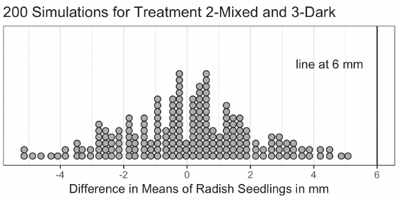
Pre-K–12 Guidelines for Assessment and Instruction in Statistics Education II (GAISE II)

88 |

the process repeated 200

times.

The observed difference of

6.2 mm was never exceeded

in this simulation of 200

re-randomizations, for an

approximate p-value of 0/200.

This gives strong evidence

against the hypothesis that

the difference between means

for Treatments 1 and 2 is due

to chance alone.

In a comparison of the means for Treatments 2 and 3, the same procedure is used: mixing the growth

measurements from Treatments 2-Mixed and 3-Dark together, randomly splitting them into two groups

of 28 and 58 measurements, recording the difference in means for the two groups and repeating the

process 200 times. The observed difference of 6 mm was never exceeded in 200 trials (see Figure 9),

giving strong evidence that the observed difference between the means for Treatments 2 and 3 is not due

to chance alone.

Interpret the Results

In summary, two pairs of comparisons of the three treatment groups show differences in mean growth that

cannot reasonably be explained by the random assignment of seeds to the bags. This provides convincing

evidence of a treatment effect—the more hours of darkness, the greater the growth of the seedling, at least

for these three periods of light versus darkness. The randomized assignment allows students to conclude

that the differences in growth were caused by the different levels of light.

This analysis is an example of multiple comparisons. To conclude that more hours of darkness causes

greater growth, two statistical investigative questions were posed and answered. However, a student in

Level C should note that the analyses conducted could be problematic. Only two pairwise comparisons

(Treatments 1 and 2 were compared; treatments 2 and 3 were compared) was done while there were

three different treatment condition pairs. To fully answer the investigative questions, students should

be encouraged to explore the remaining pairwise comparison. Students beyond Level C can also explore

potential pitfalls of multiple comparisons with a pairwise approach. More advanced methods exist but are

outside the scope of Level C. Such methods may be found in college-level courses.

Students should be encouraged to delve more deeply into the interpretation, relating it to what is known

about the phenomenon or issue under study. Why do the seedlings grow faster in the dark? A biology teacher

might discuss how the plants have adapted to germinate into the light (above ground) as quickly as

possible. The seedling cannot photosynthesize in the dark and is using up the energy stored in the seed to

power the growth. Once the seedling is exposed to light, it shifts its energy away from growing in length

to producing chlorophyll and increasing the size of its leaves. These changes allow the plant to become

self-sufficient and begin producing its own food. Even though the growth in length of the stem slows, the

growth in diameter of the stem increases and the size of the leaves increases. Seedlings that continue to

grow in the dark are spindly and yellow, with small yellow leaves. Seedlings grown in the light are a rich,

green color with large, thick leaves and short stems.

Figure 9: Re-randomization distribution for the difference in means of

Treatment 2-Mixed and Treatment 3-Dark

Level C

| 89

Example 5: Considering Measurements when Designing Clothing –

Linear Regression

Formulate statistical investigative questions

Clothing designers must create patterns for clothing that are likely to fit their buyers. For clothing to fit

people appropriately, a designer must understand the relationship between the dimensions of various

physical features. For example, a shirt designer must take into consideration the length of a person’s arm

in relation to the length of their torso. Suppose a statistics class was tasked with creating a pattern for

the costumes for the chorus of the school play. The costumes consist of cloaks that run all the way to

the ground, so an actor’s feet would not be showing. The cloaks are designed so that the forearm sleeve

fits tightly around the arm, running from the elbow to the hand. They ask the following statistical

investigative question:

How does a person’s forearm length relate to their height? Can forearm length be used to predict height?

Collect/Consider Data

Students in the statistics class decide to use their own body measurements to help them make the

cloak pattern. They take their own measurements at home to avoid any potential sensitivity issues in

class. Level C students should recognize that taking measurements from students in their class might

not be generalizable to the school, however, it offers a basis for their pattern cutting. An important

consideration here is to agree on the

definition of “forearm” before begin-

ning to take measurements. The

cloak forearm is determined to be the

measurement from the crease of the

elbow on the inside of the arm to the

end of the wrist. The data obtained

by the students (in centimeters) are

provided in Table 7. Each row rep-

resents a student.

Students are sometimes unfamiliar

with metric units and might want

to examine the data in more familiar

units. To do this, the data can be

transformed. Using dimensional

analysis, new variables can be created

that transform the units from cm to inches, by multiplying the “old” values by 0.393701 in/cm (or

dividing by 2.54 cm/in).

Analyze the Data

A good first step in any analysis is to plot the data (see Figure 10). The scatterplot indicates that a linear

trend would be a reasonable model for summarizing the relationship between height and forearm length. In

Level B, the Quadrant Count Ration (QCR) was considered as a numerical summary for quantifying the

Table 7: Heights vs. Forearm Lengths

Forearm (cm) Height (cm) Forearm (cm) Height (cm)

45.0 180.0 41.0 163.0

44.5 173.2 39.5 155.0

39.5 155.0 43.5 166.0

43.9 168.0 41.0 158.0

47.0 170.0 42.0 165.0

49.1 185.2 45.5 167.0

48.0 181.1 46.0 162.0

47.9 181.9 42.0 161.0

40.6 156.8 46.0 181.0

45.5 171.0 45.6 156.0

46.5 175.5 43.9 172.0

43.0 158.5 44.1 167.0

Pre-K–12 Guidelines for Assessment and Instruction in Statistics Education II (GAISE II)

90 |

strength of the relationship between

two quantitative variables. The QCR

was based on a count of points in

each of the four quadrants of the scat-

terplot defined by the mean lines for

each of the two variables. In Level C,

the analysis evolves to using Pearson’s

correlation coefficient (r) that takes

into account the distance of the points

from the mean lines. The mean lines

are a vertical and a horizontal line

placed at the mean of the forearm

measurements and the mean of the

height measurements, respectively.

Similar to the QCR, Pearson’s r is

unitless and is always between –1 and

+1, inclusive. See Kader and Franklin (2008) for a more detailed discussion. Pearson’s r for these data

obtained from technology is 0.8. This indicates that there is a strong positive linear association between

height and forearm length.

If the “cloud” of points in a scatterplot has a linear shape (a narrow oval or sausage-like pattern in contrast

to a more circular pattern), a straight line may be a realistic model of the relationship between the variables

under study. Level C students should be introduced to the least-squares regression line (referred to

throughout this example as the least-squares line), which is the line that minimizes the sum of the squared

residuals. Residuals are defined to be the deviations in the y-direction between the points in the scatterplot

and the least-squares line. Applets can be used to show the concept of the least-squares line and residuals.

The least-squares line also runs through the point where the mean lines cross at (mean x, mean y) of the

cloud of points.

The equation for the least-squares line for this relationship (calculated with statistical software) shown in

the scatterplot in Figure 11 is:

Predicted Height = 45.8 + 2.76(Forearm Length).

The plot below the scatterplot shows the residuals (Figure 11).

The residuals show variation around the least-squares line, as measured by the standard deviation of the

residuals.

Students in Level C should evaluate whether the linear model is appropriate and a good fit. The residual

plot reveals that there are no patterns: there are similar amounts of negative and positive residuals and they

are both negative and positive across the values of x. This supports the initial impression of the scatterplot

that the linear model is appropriate. The correlation coefficient was already noted above as being high

(0.8), indicating the linear relationship is strong.

Figure 10: Scatterplot with no regression line

Level C

| 91

The slope (about 2.8) of the least-squares line

can be interpreted as an estimate of the average

difference in heights for two persons whose

forearms are 1 cm different in length. That is,

if one actor’s forearm length is 1 cm greater

than another, the actor is expected to need a

cloak that is about 2.8 cm longer. The intercept

of 45.8 centimeters can theoretically be

interpreted as the expected height of a person

with a forearm zero centimeters long. Yet

this is clearly unreasonable, so in this context

interpreting the y-intercept of the least-squares

line is not sensible. However, the least-squares

line can reasonably be used to predict the

height of a person for whom the forearm length

is known, as long as the known forearm length

is in the range of the data used to develop the

least-squares line (39 to 50 cm for these data).

For example, the predicted height of someone

with a forearm length of 42 cm would be:

Predicted Height = 45.8 + 2.76(42) =

161.7cm

When using a fitted model to predict a value of y (the response variable) from x (the explanatory variable),

the associated prediction interval depends on the standard deviation of the residuals. This is not to be

confused with a confidence interval for a mean response. The standard deviation of the residuals can be

used to create a prediction interval for the height of all high school students with a forearm length of 42.

Thus, for a randomly selected high school student with a forearm length of 42cm, it is predicted that

they will have a height in the range from 150.1cm to 173.3cm. This prediction interval is calculated by

adding and subtracting 2*(standard deviation of the residuals) to the predicted height value. This assumes

that the distribution of heights for high school students with a forearm length of 42cm is bell-shaped.

For these data, the standard deviation of the residuals is 5.8 (not shown here, but provided as part of the

computer output), so 2*(standard deviation of the residuals) = 2*(5.8) = 11.6 cm. Adding and subtracting

this amount from the predicted height of 161.7 gives a prediction interval for the height of a student with

a forearm length of 42cm from 150.1 to 173.3 cm.

Interpret the Results

Students in the statistics class conclude that forearm length and height are linearly related and forearm

length might be used to predict height. For example, for a specific forearm length of 42 cm, they should

be reasonably confident the individual heights of the high school students will be between 149.5cm to

174.2cm. This is a fairly wide interval (just under 10 inches), which suggests that while they might use

the regression equation to predict the height, they should expect quite a bit of variation and so perhaps

will need to do much hemming.

Figure 11: Least-Squares Line and Residual plot

Pre-K–12 Guidelines for Assessment and Instruction in Statistics Education II (GAISE II)

92 |

Example 6: Napping and Heart Attacks – Inferring Association from an

Observational Study

Formulate statistical investigative questions

The effect of napping (whether taking naps or not) on cardiovascular disease (CVD) such as heart attacks

is uncertain. Some studies have indicated a positive effect of napping, some a negative, and some no effect.

However, many of these studies did not consider napping frequency. A statistical investigative question

to consider is:

Is there an association between napping frequency and CVD?

Collect data/Consider data

Observational studies are often the only option for situations in which it is practically impossible or

unethical to randomly assign treatments to subjects. Such situations are a common occurrence in the

study of causes of diseases. As researchers consider how to design a study to answer this statistical inves-

tigative question, it would be impossible to randomly assign subjects to treatment groups telling subjects

they cannot take weekly naps, to take exactly 1-2 weekly naps, or to take more weekly naps and then trust

subjects to honor those number of weekly naps for a long observation period.

Instead, researchers in Switzerland

(Hausler, Haba-Rubio, Heinzer R,

Marques-Vidal, P., 2019) designed

an observational study following

3,462 Swiss subjects who had no

previous history of CVD. The

subjects were asked to self-report

their typical nap frequency during a

week. The researchers then classified the subjects into four groups OF the explanatory variable. No nap,

1-2 weekly, 3-5 weekly, 6-7 weekly. The response variable was whether or not (yes or no) the subject had

a CVD event during the next 5 years. Table 8 shows the summary counts of subjects for the categories of

the explanatory and response variables at the end of the 5-year period.

Analyze the Data

Understanding the nature of the counts in Table 8 is essential for analyzing the data. Each observation is

accounted for in one of the interior cells that show joint frequencies (where categories for the two variables

overlap). Additionally, each observation is one of the total 3462 observations as well as one of the row

marginal frequencies and one of the column marginal frequencies. For example, a subject who is classi-

fied as no nap and no CVD event is one of the 1921 joint frequency number and also one of the 3307

subjects who had no CVD and one of the 2014 subjects who do not nap. Analysis of the table might lead

students to examine whether there is a noticeable difference in the percentage of subjects who had a CVD

event for each napping frequency category. For example, out of the subjects who took no weekly naps, the

percentage who had a CVD event was 93/2014 = 4.6%. Of those subjects who took 1-2 weekly naps, the

percentage who had a CVD event was 12/667 = 1.8%. Table 9 displays all these conditional percentages.

Table 8: Nap Frequency and CVD event

Nap Frequency

CVD event No nap 1-2 weekly 3-5 weekly 6-7 weekly TOTAL

Yes 93 12 22 28 155

No 1921 655 389 342 3307

TOTAL 2014 667 411 370 3462

Level C

| 93

Table 9: Conditional Percentages on CVD event for each Nap Frequency

Nap Frequency

CVD event No nap 1-2 weekly 3-5 weekly 6-7 weekly TOTAL

Yes 4.6% 1.8% 5.4% 7.6% 4.6%

No 94.4% 98.2% 94.7% 92.4% 94.4%

TOTAL 100% 100% 100% 100% 100%

The different napping groups

show differences in percentages

for the incidence of a CVD

event. The 1-2 weekly group had

the lowest incidence percentage

at 1.8%, which was at least 3

percentage points lower than

that of the other three napping

groups. The group who took no

naps had an incidence percentage

of 4.6%. The group of subjects

who took 6 - 7 weekly naps had

the highest percentage of CVD

events at 7.6%. These results

are shown in the percentage bar

graph in Figure 12.

Descriptively, it appears that those who took no naps are at moderate risk of CVD within 5 years, those

who take 1-2 naps are at the lowest risk, and the risk increases the more naps the person took. (We’re using

the conditional percentage of having a CVD given the number of naps as a measure of risk.) But could this

association be due merely to chance? In other words, might there be no relationship between the number

of naps and the occurrence of CVD?

One approach is a Chi-squared

test, which compares the number

of counts actually observed in each

cell with the number of counts

expected in each cell if there were

no association between the two

variables. Whereas understanding

the technical underpinnings of

Chi-squared tests are beyond Level C, students can use technology and interpret the results in context.

The expected values can be computed by using the marginal percentages (CVD Yes = 155/3462 = 4.48%;

CVD No = 3307/3462 = 95.2%) and multiplying them by the column totals resulting in the following:

Figure 12: Conditional Percentages for CVD event = Yes

Table 10: Expected values based on conditional percentages

Nap Frequency

CVD event No nap 1-2 weekly 3-5 weekly 6-7 weekly TOTAL

Yes 90.17 29.86 18.40 16.57 155

No 1923.83 637.14 392.60 353.42 3307

TOTAL 2014 667 411 370 3462

Pre-K–12 Guidelines for Assessment and Instruction in Statistics Education II (GAISE II)

94 |

The Chi-squared statistic is 20.3

with a p-value of 0.0001 and 3

degrees of freedom.

Interpret the results

The Chi-squared test resulted

in a p-value of 0.0001. There

is a 0.01% probability of get-

ting a Chi-square test statistic

of 20.3 or larger if what is being

observed is due solely to chance

under the presumption of no

association. Therefore, there is

convincing evidence to conclude there is an association between the number of naps taken and the occur-

rence of CVD. Note that the chi-squared approach does not provide information about the direction of

the association; it doesn’t tell whether more naps is associated with an increased risk or a decreased risk. In

fact, from considering the bar chart, the association may be non-linear. The risk is higher for those taking

no naps than for those taking 1-2 naps weekly, and the risk then increases as the number of naps increases.

The risk for the no-nap group compared to the 1-2 naps weekly group could be measured by the relative

risk (RR) computed as RR = 4.6%/1.8% = 2.55. We can interpret this to mean that the percentage of

CVD events is 2.55 times larger for no nappers than for 1-2 weekly nappers.

Does this study imply everyone should start taking 1-2 naps a week to avoid CVD events and not take

more than 2 naps a week? Not necessarily, because this was an observational study, a cause-and-effect

statement cannot be made. There may have been some confounding variables other than nap frequency

impacting the response variable of CVD event. For example, if older people are more likely to take 6-7

naps per week and are also more likely to have CVD, then the variable of age might be important to

consider. In this instance, there would be an association between napping frequency and CVD even if

napping has no effect on CVD. Likewise, if people with other health issues are more likely to nap and

more likely to have CVD, then having other health issues is confounded with napping frequency.

When experiments cannot be conducted and observational studies are used instead, it is important to

identify potential confounding variables. Then, if possible, control for these variables. One way to do

this is to disaggregate the data to analyze the explanatory and response variables by the categories of the

confounding variable. As students advance beyond Level C, they will learn more about how to control for

potential confounding variables with the design of the study. They will also learn more formal statistical

methods for analyzing the data, such as confidence intervals for differences, and how to judge the practical

importance of the association by evaluating effect sizes.

Example 7: Working-age Population – Working with Secondary Data

Formulate statistical investigative questions

Students and the general public routinely encounter statistical graphics that are rarely seen in Pre-K–12

classrooms. Part of statistical literacy is being able to grapple with data presented in the media using vari-

ous unconventional representations.

Figure 13: Chi-squared results from applet

Level C

| 95

The New York Times has a weekly feature, What’s Going On in This Graph? (WGOITG) (https://

www.nytimes.com/column/whats-going-on-in-this-graph) that provides excellent examples of such

graphics. Each week, a statistical graphic that appeared in an earlier story is presented with

some context removed. Students are invited to post responses to three prompts: What do you

notice? What do you wonder? What’s going on in this graph? Alternatively, students might be asked to

write a catchy headline that captures the graph’s main idea.

For example, one WGOITG was on the topic of changes in the size of the working-age population

over a 10-year period. In a context such as this, posing an answerable statistical investigative question is

the primary focus. After examining this particular graph, students might pose the following statistical

investigative question:

How has the working-age population shifted across the United States?

Collect data/Consider data

The graphic given in WGOITG is a heat map, which represents a statistical analysis of the data. The leg-

ends provided by the analyst help us understand the data themselves. The graph color-codes each county

in the United States according to the shift in the working-age population. The graph was converted to

grayscale for this publication. For example, a county is colored dark grey if the population of working-age

people (defined as 25 to 54 years old) has decreased by more than 10% from 2007 to 2017. On the other

end of the color spectrum, a light grey color represents a county that has increased in the working-age

population by over 10% from 2007 to 2017.

Figure 14: Heatmap of the United States showing change in population.

Source: The New York Times’s What’s Going On in This Graph? September 19, 2019

Pre-K–12 Guidelines for Assessment and Instruction in Statistics Education II (GAISE II)

96 |

Students in Level C need to study summarized secondary data provided in graphics in order to understand

the multiple variables being displayed. Level C students should be able to identify the observational units

(counties) and all variables represented in this graph. For example, one variable represented is the percent

change in the number of people aged 25-54 years who reside in a county. The data set that produced these

graphics might have had columns labeled “county”, “working_age_population_2007”, “working_age_

population_2017”, “percent_change”.

Analyze the data

In this case, the analysis has been done. The graphic is the analysis of the data. This is typical when inter-

preting others’ work as it appears in news media or scientific publications.

Interpret the Results

Level C students may notice that the middle and north-eastern parts of the country are predominantly dark

grey, suggesting a decrease in the working-age population in those parts of the country, while the west and

south have tended to see an increase in the working-age population. Overall, the data suggest large shifts over

time in the number of working-age individuals. Students might also comment on the within-state variability.

Some states, such as Nebraska, Maine, or Vermont, are almost entirely dark grey, indicating that the entire

state suffers from a decrease in the working-age population. Other states, such as Utah, are mostly light grey,

indicating large increases in the working-

age population. Other states, such as

Texas and California, have more variabil-

ity; some areas of the state see increases

while others see declines.

Level C students might also consult

other sources of information to help

interpret their results. The WGOITG

heat map pictured above captures the

difference over one decade without

considering the month-by-month

or year-by-year time increments.

Considering the monthly data provides

an opportunity to further interrogate

the data. The time series graph (Figure

15) shows the number of working-

age individuals in the entire United

States for each month from January

2007 through December 2017. The

working-age population declined

overall through 2014 and then appears

to have been increasing since 2015.

A Level C student might notice the

pattern in the timeplot where there is

a drop from the end of one year to the

beginning of the next (e.g., the count

in Dec 2007 is about 126 million but

Figure 15: Timeplot of the monthly data from the heatmap

Figure 16: Timeplot with a moving average added

Level C

| 97

falls in January 2008 to less than 125.5 million). Students might speculate that the age of a person was

calculated based on their birth year rather than birth month. In order to account for this but not lose

the level of detail available in the monthly data, they can compute a moving average. Moving averages

can vary in the time period used (e.g., 3-months, 6-months, etc.); in this case, it makes sense to use a

12-month moving average, which will smooth out these annual adjustments. The graph in Figure 16

includes the monthly data as well as the 12-month moving average.

If monthly data from 2007 to 2017 are available, the first 12-month moving average that can be calculated

is for June 2007 (includes Jan 2007 to Dec 2007) and the last value that can be calculated is for June 2017

(includes Jan 2017 to Dec 2017). The moving average has a similar but smoother trend. There are other

ways to smooth patterns of graphs, such as seasonality adjustments and exponential smoothing.

Example 8: Classifying Lizards – Predicting a Categorical Variable

Formulate Statistical Investigative Questions

Level C students go beyond Level B by tackling more open-ended questions and by considering datasets

that might require some preparation before analysis. Data sets appropriate for Level C may have addi-

tional variables that are not used in the analysis, forcing students to consider different aspects of the data

and how multiple pathways might be productively pursued.

Suppose that students in a science class are exploring the impact of human development on wildlife. In an

earlier analysis, students discovered that lizards in “disturbed” habitats (habitats with substantial human

development) tended to have greater mass than lizards in natural habitats. Students posed this statistical

investigative question:

Can a lizard’s mass be used to predict whether it came from a disturbed or a natural habitat?

Students can approach this statistical investigative question by trying to define rules for how a randomly

selected lizard can be classified as coming from either a disturbed or natural habitat.

Collect data/Consider data

A biologist captured a number of individuals from one species of lizard, Anolis sagrei, across two different

habitat types on each of four islands in the Bahamas. The data was collected by Erin Marnocha during her

time as a graduate student at the University of California Los Angeles. The lizards were selected through

a random sampling procedure. Some of the lizards lived in habitats that were developed by humans (dis-

turbed) while others lived in natural habitats with no human development (natural).

A total of 160 lizards were captured, 81 from natural habitats and 79 from disturbed habitats. Once

captured, the lizards were measured across several physical characteristics, including their mass, length,

breadth, foot span, head width, etc. Lizards captured from habitats with human development were labeled

“disturbed” and those captured from habitats without development were labeled “natural.”

The first few rows of the data are given in Figure 17. Note that the data are displayed in long format where

each row represents a lizard, and the columns tell us the measured characteristics of the lizard.

To consider and understand these secondary data, Level C students can examine and query the dataset

using technology. Level C students should note that although there are 160 lizards included in the data

Pre-K–12 Guidelines for Assessment and Instruction in Statistics Education II (GAISE II)

98 |

set, quite a few of them have missing values for one variable or another. The “Tail length” variable is

missing quite a few values (for example, see Index 3 in Figure 17). Students with experience catching

lizards will know why: lizards can lose their tails to help evade capture.

Figure 17: Beginning of lizard data in long format

This statistical investigative question relies on only two variables: “Habitat” and “Mass” (measured in

grams). For ease of analysis, students might create a new data set that contains only those two variables.

Analyze the Data

A comparative dotplot of the mass (Figure 18) shows considerable overlap between the two types of

habitats. The statistical investigative question focuses on predicting whether a randomly selected lizard

comes from a natural or disturbed habitat (categorical response variable) using the mass of a lizard as the

explanatory variable. In Level C, students can approach the analyses using classification (beyond Level C,

several additional modes of analyses exist to help answer such statistical investigative questions).

A classification approach essentially requires students to propose a rule based on the mass of the lizard

that predicts the type of environment the lizard came from. For example, consider a potential rule that

classifies lizards <6.25 g to be from natural habitats (“natural”). Students in Level C can analyze whether

this provides a good prediction rule.

The dotplot shows that if lizards weighing less than 6.25g are classified as from natural habitats then 100%

of these lizards are correctly classified (because all of these lizards in our sample weigh less than 6.25g).

However, this is not a perfect classification rule, because a high percentage (53/79 = 0.671 = 67.1%) of the

lizards that are from disturbed habitats would be misclassified because they weigh less than 6.25 g. Since

the dotplots show a lot of overlap in the masses of the two groups, the classification of a lizard as coming

from a disturbed or a natural habitat will not be straightforward.

Level C students should recognize that less overlap between distributions provides a greater classification

success rate. Also, changing the cut-off point can vary the misclassification rate. For example, if lizards with

mass less than 5.0 g are classified as “natural,” fewer errors will be made when encountering lizards that

are truly from disturbed habitats, but more errors will be made with lizards from truly natural habitats.

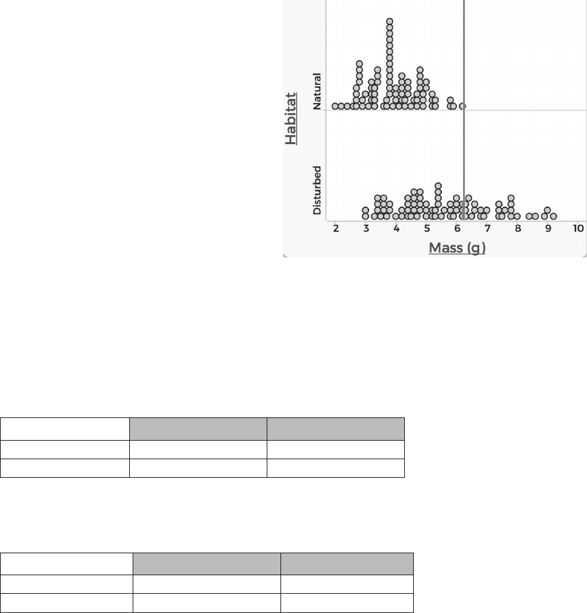
Level C

| 99

Analyzing the data using a classification

approach is obtainable for Level C students.

With appropriate technology or careful

counting of dots in the dotplot, students can

compute and interpret a confusion matrix

for any cut-off rule they choose. A confusion

matrix shows the true values in the columns

and the classification categories in the rows

(or vice versa). Thus, the upper-left cell of

the matrix below indicates that 26 lizards

were correctly classified as belonging to a

disturbed habitat. A perfect classifier will

have 0’s on the off-diagonal.

The first confusion matrix in Table 11

shows the results of classifying with the rule

where lizards with mass less than 6.25 g are

classified as “natural.” All 81 of the lizards from natural habitats were classified as natural, but 53/79

lizards from disturbed habitats were incorrectly classified. Overall, the misclassification rate is (number of

lizards misclassified)/ total number of lizards = (53 + 0)/(26+53+0+81) = 0.331 or about 33%.

Table 11: Confusion Matrix for mass < 6.25 g

Truly from Disturbed Habitat Truly from Natural Habitat

Classified as “disturbed” 26 0

Classified as “natural” 53 81

By changing the rule to classify a lizard as natural if its mass is less than 5 g, a new confusion matrix results:

Table 12: Confusion Matrix for mass < 5 g

Truly from Disturbed Habitat Truly from Natural Habitat

Classified as “disturbed” 49 11

Classified as “natural” 30 70

Now the number of misclassified lizards is 30+11 = 41. Therefore the misclassification error rate

is (30 + 11)/(49+30+11+70), or about 26%. The new rule improves on the previous rule.

Students can continue to explore classification rules to determine which produces the lowest misclassification

rate.

Determining an optimal procedure for classification is beyond Level C. Instead, students in Level C should

understand how changes in a rule affect misclassification rates by computing probabilities. Level C students

should understand that a classification approach can be used to answer statistical investigative questions

that focus on predicting a response variable that is categorical by using another variable. Beyond Level

C, several other approaches exist to help answer such questions (e.g., logistic regression, random forests,

machine learning, and deep learning algorithms). In general, classification is part of prediction—here, for

example, one is trying to predict the category of a randomly selected lizard based on one or more variables.

These methods are often discussed in the news, especially with the advances in machine/deep learning. For

Figure 18: Stacked dotplots showing mass of 6.25 g

as cutoff

Pre-K–12 Guidelines for Assessment and Instruction in Statistics Education II (GAISE II)

100 |

example, facial/image recognition is an advanced example of a classification problem prevalent in the media

today (e.g., https://www.nytimes.com/2019/12/19/technology/facial-recognition-bias.html). To promote

statistical literacy, students should learn the basic ideas of classification approaches in Level C.

At Level C, given data about a new lizard from the population, students should be able to classify the lizard

and provide the probability of misclassification for that new observation.

Interpret the Results

A misclassification rate of 26% might strike some students as good and others as not-so-good. Students

might wonder how to evaluate misclassification rates. To find a “baseline” rate for comparison, one

approach is to ignore the mass of a lizard and classify all lizards into the largest group. Because there are

79 lizards from disturbed habitats and 81 from natural habitats, all lizards can be classified as “natural”

habitats without looking at their mass.

This rule will misclassify all of the lizards from disturbed habitats, so the misclassification rate will be 79/

(81+79) = 0.49 or 49%. By comparison, the previous classification rule with a 26% misclassification error

rate (lizards with a mass of less than 5.0 g are “natural”) is quite a bit better than this baseline rate.

Because these lizards were randomly sampled, these misclassification rates can be interpreted as estimates

of the proportion of incorrect classifications for future captured lizards, as long as they are captured from

the same population as the lizards in this dataset. Level C students can conclude that, in fact, lizards can

be classified based on their mass in such a way that the probability of misclassification is lower than if they

had been simply classified as all belonging to the same habitat.

Analysis Revisited

The previous approach depends on a single explanatory variable – mass of the lizard. How might multi-

ple variables be used to classify the lizards? More specifically, the statistical investigative question can be

rephrased as:

Can a lizard’s mass, head depth, and hind limb length be used to predict whether it came from a disturbed or

a natural habitat?

One approach that furthers the simple classification approach which is accessible to Level C students if

they have the appropriate technology is to apply a Classification and Regression Tree (or CART). CART

is an example of a modern statistical approach that relies on an algorithm, rather than a mathematical

model. An “algorithm” in this case is taken to mean a series of rules.

Although applying and interpreting the CART algorithm is accessible to Level C students, the details of

the algorithm are not necessary for students to begin their understanding. CART begins with splitting the

data according to a rule. Suppose the rule is the one above: classify a lizard as natural if its mass is less than

5g. This rule splits the data into two groups.

One group consists of lizards less than 5 g that are classified as “natural” (even though this group may

contain some that are not from the natural habitat), and the other group consisting of lizards larger than

5 g that are classified as “disturbed” (even though some may not be from the disturbed habitat).

Level C

| 101

Students can then consider the group of

lizards classified as “natural” and determine

if, based on one of the variables in the data

set, they can further split this group into two

smaller groups.

For example, the initial classification split

classified 100 lizards as “natural” because

their mass was less than 5 g (this can be

seen in the confusion matrix in Table 12 as

30+70=100). Now, considering only these

100 lizards, students can repeat the process

with a new variable, for example by making

stacked dotplots of the 100 lizards’ head

depth measurement. The lizards truly from

a disturbed habitat would be plotted on top

and the natural lizards below. The result is

shown in Figure 19.

Again, students can consider different “cutoff” values. A first attempt might be to draw a cutoff at a head

depth of 5.25 mm, since visually that seems to separate the bulk of the data on the left from the remaining

data on the right. Because the natural lizards have a slightly larger mean head depth, students may classify

lizards to the right of the cutoff line shown in Figure 19 as “natural,” and those to the left as “disturbed.”

This results in a new set of classification rules:

1) If the mass is less than 5 g, consider the head depth. If the head depth is less than 5.25 mm, classify as

“disturbed.” If the head depth is greater than or equal to 5.25 mm, classify as “natural.”

2) If the mass is greater than or equal to 5 g, classify as “disturbed.”

The next step would be to repeat this procedure on the 60 lizards whose mass was greater than or equal to

5 g and who were thus classified as “disturbed.”

This process can continue for quite a while. At each step, any variable may be considered in order to split

the data into two classification groups. The CART algorithm does what no human would be patient

enough to do. At each step of the process, it considers all available variables and all possible cutoff values.

It determines which provides the lowest misclassification rate, and then it splits the data based on that

rule. This creates two new groups, and the process is repeated on those two groups. This, of course,

produces four groups, and the process is repeated on each of those four new groups. The process stops

when performing a split provides no improvement in the misclassification rate or when a group is too

small to split.

The result could be written as a series of rules, but it is better visualized as a tree. Figure 20 shows the

CART for these data. Each split contains a rule stated as a condition. If the condition is true, move down

the left branch and continue in this fashion until reaching an end node. The node indicates how to classify

the observation.

Figure 19: Stacked boxplots for 100 lizards with mass

less than 5 g showing 5.25 cm head depth as a cutoff

Pre-K–12 Guidelines for Assessment and Instruction in Statistics Education II (GAISE II)

102 |

For example, consider a lizard with

a mass of 4.5 g, head depth of 5

mm, and a hind limb measurement

of 11 mm. The first rule (mass ≥

5.35 g) does not apply to this lizard,

so this tells a student to move to

the right branch. The next rule

considers head depth, and because

the lizard’s head depth is not less

than 4.25 mm, a student can again

move to the right. Next, the mass

is considered again, and since it is

greater than 4.25 g, this time the

move is to the left. Finally, because

the hind limb measurement is less

than 12.65 mm, the move is to

the left, which classifies this lizard

as “disturbed.” Had the hind limb

length been greater than 12.65 mm this lizard would have been classified as “natural.”

The numbers below the classification label indicate the number of lizards of both types that were classified

with that category label. For example, in the end node shared by our hypothetical lizard (Disturbed 9/1),

nine of the lizards from our sample data who were sent to that node were truly from a disturbed habitat,

and one was truly from a natural habitat. So, for lizards with traits similar to these, the misclassification

rate is 1/10, or about 10%.

Interpret the Results

Each split of the tree is a decision, and each lizard will be classified according to the end-nodes of the tree.

Of the two numbers in each node, the number on the left represents the number of lizards truly from

disturbed habitats, and the number to the right is truly from natural habitats. For example, the left-most

node classifies lizards as disturbed. This classification is correct for 42 lizards and incorrect for 4 lizards.

The overall misclassification rate for this tree is 18% (27 out of 160 lizards), a figure computed by the

software that produced the tree. We could confirm this by counting the number of misclassifications and

dividing by 160, the total number of lizards. For example, the left-most node is labeled as “Disturbed”

and contains 42 lizards from disturbed habitats and 4 from natural habitats, and thus there are

4 misclassifications. Continuing left to right, theare are an additional 1, 1, 11, 3 and 7 misclassifications

for a total of 27 misclassifications out of 160 lizards. This gives the misclassification rate of 27/160 or

about 18%. This tree improves upon the earlier classification rule, which was based solely on mass.

If technology is not available to create trees, students can still benefit from creating their own trees using

sets of rules of their own design.

Summary of Level C

Students at Level C should become adept at using questioning throughout the statistical problem-solving

process. In Level C, statistical investigative questions expand from summative and comparative situations

to include questions about associations and relationships among multiple variables, including predictions.

Figure 20: CART Tree for Lizard data where the left branch is

taken when rule applies.

Level C

| 103

Once an appropriate plan for collecting data to answer a statistical investigative question has been imple-

mented and the resulting data are in hand, the next step usually is to summarize the data using tools such

as graphical displays and numerical summaries.

At Level C, students should be able to select data analysis techniques appropriate for the type of data

available, produce descriptive statistical analyses, and describe in context the important characteristics

of the data. Level C students should be able to provide more sophisticated and insightful interpretations

compared to Levels A and B. These interpretations should integrate the context and objectives of the

investigation to draw conclusions from data and to support these conclusions using statistical evidence

(both descriptive and inferential).

Level C students should see statistics as providing powerful tools that enable them to answer statistical

investigative questions and to make informed and trustworthy decisions. Students also should understand

the limitations of conclusions based on the data from sample surveys and experiments, and they should

be able to quantify the uncertainty associated with these conclusions using margin of error and related

properties of sampling distributions. Statistically proficient students at Level C are “healthy skeptics” of

statistical information, capable of asking questions to assess the validity of statistical findings. At the same

time, they are cognizant of the power of statistical analyses to find information and meaning in data. Level

C students should understand that because their own work will be read by others, they should carefully

document both their data and their analyses so that others can reproduce their analysis. Level C students

should understand the ethical consequences of their experiments and analyses.

While Level C rounds out students’ statistical literacy, students should understand that more complex

statistical investigative questions, data collection methods, study designs, and analysis methods exist.

Beyond Level C there is an additional wealth of statistics to be learned. Levels A, B, and C material

provides students with the basics of statistical literacy at this point in time. The material will continue to

evolve, however. It is not just data that is changing, it is processes, technology, philosophies, strategies, and

many other changing facets that lead to the evolution of statistical methods. Statistics is not a stagnant

discipline; instead, it is an evolving field that is rooted in the statistical problem-solving process discussed

in this report.

| 105

Assessment

Assessments provide feedback to learners, teachers, and guardians by providing a gauge of what students

know and can do at a particular point in time. It is essential that instruction and assessment be aligned,

consistent with the principles outlined in the different Levels in GAISE II. Assessments of students’ statistical

thinking should assess conceptual understanding, be set in a context, and require interpretation (Peck, Gould

& Miller, 2013). These criteria apply to formative and summative assessments regardless of the form of

assessment (e.g., discussions, activities, projects, reflective essays, homework problems, tests). While it may

not be feasible to assess statistical reasoning at all stages of the statistical problem-solving process in a single

item, it is important to construct items that assess multiple parts of the process across time.

Many statistics items commonly found on standardized or locally developed assessments require lower-level

cognitive skills (such as recall) and focus on procedures and definitions. In addition, many of these items do

not focus on statistical reasoning but rather focus on mathematical computations. For example, a task asking

students to find the mean for a set of numbers is a low-level task that involves mathematical computation

and no statistical reasoning. Even a task that involves giving students all but one data point and the mean and

asking them to find the missing data point is a lower-level mathematics task. Fortunately, there are several

examples of robust assessment items on standardized assessments as well as resources for teachers to find such

items for classroom use.

National and International Standardized Assessments

Several national and international standardized assessments include a focus on data analysis and statistics.

For instance, the Programme for International Student Assessment (PISA), which is given to 15-year-old

students around the world to assess ability to apply knowledge to real-world situations, is expected to focus

on mathematics in 2021 with computer simulations and conditional decision making identified as topics

for special emphasis. According to the College Board, 29% of the items on the mathematics portion of the

SAT address problem solving and data analysis (which includes proportional reasoning and probability).

Data analysis, statistics, and probability is one of five content strands assessed on the National Assessment

of Educational Progress (NAEP). And, of course the Advanced Placement (AP) Statistics Examination

contains only questions about statistics. The standard exam format includes 40 multiple-choice questions,

five short free-response problems, and 1 investigative task, and over the years it has progressed to have an

emphasis on conceptual understanding and interpretation rather than simply on arithmetic calculation.

Selected items are released after each administration and are available to teachers.

Sources of Quality Items for Educators

Creating high quality assessment items is time-consuming and challenging. Thus, we profile two sources

that have been vetted and can serve as resources for teachers – Levels of Conceptual Understanding in

Statistics (LOCUS) and Statistics Education Web (STEW).

LOCUS

The LOCUS assessments are based on the original GAISE I framework, aligned with the Common Core

State Standards, and constructed as reliable measures of understanding across the levels of development

Pre-K–12 Guidelines for Assessment and Instruction in Statistics Education II (GAISE II)

106 |

and throughout the statistical problem-solving process. Both multiple choice and constructed response

questions are included, and there are different versions of the assessments based on the different GAISE

Levels. Each version has equated forms for pre/posttest purposes, so they can be used for both formative

and summative assessments.

Both types of questions, multiple choice and constructed response, can be viewed by grade level or by

component of the statistical problem-solving process. Multiple choice sample questions include associated

standards, student performance, correct answers, and commentaries. Constructed response questions

include the additional information of scoring rubrics, common misunderstandings, sample responses,

and resources.

STEW

STEW online resource includes peer-reviewed lesson plans. STEW lesson plans follow a standard format

and include objectives, applicable Common Core State Standards, and instructions for enacting the lesson

in the classroom. Although they are sorted by grade level, many lessons can be modified to address similar

content at different levels. Material may also include problems with sample solutions, slides that can be

used to guide class discussions, and directions for technology tools. Educators are encouraged to use the

lesson plans that are on this site as well as contribute new lesson plans that they have found effective in

their classrooms. These lessons could be adapted to assessments.

Some of the following examples of assessment items are from the resources mentioned (e.g., LOCUS and

STEW) and they are provided by Level in the following sections. These examples are meant not to be

exhaustive but instead showcase how statistical thinking can be assessed.

Level A Assessment Examples

Example 1: Measures of center

The students in Ms. Kieffer’s class kept track of how many children in their class ate school lunch during

the month of February. Table 1 shows what they found:

Table 1: Number of children eating a school lunch

M T W Th F

18 21 19 20 22

25 17 19 18 19

19 20 21 21 23

21 20 23 19 23

If the principal asked you approximately how many people in your class ate the school lunch each day, what

would you tell her? Explain how you obtained your answer.

Assessment

| 107

Example 2: Variability, sampling, and drawing inferences

I want to know what the favorite food is of people in the world. Would I get a reasonable answer if I used your

class as a sample? Why or why not?

Example 3: How to model data in a variety of ways to see how the

conclusions drawn are inuenced by the way the data are represented

(from “Candy Judging” Lesson Plan on STEW website)

Jeremy’s class rated the chocolate candies from most favorite (1) to least favorite (4). His class data are

recorded and shown in Table 2.

Use the approaches below to determine the class favorite.

(a) Find the chocolate that was selected as favorite (ranked with a 1) the most often.

Represent this data in a picture graph (or dotplot). Which candy would represent the class favorite if

this method were used to determine the favorite?

(b) Find the chocolate that was selected as least favorite (ranked with a 4) the most often.

Represent this data in a picture graph (or dotplot). Which candy would represent the least favorite of

the class if this method were used to determine the least favorite?

scores was used to determine the favorite? Which chocolate would be the least favorite using this method?

(d) Find the median score of each type of chocolate. Which chocolate would represent the favorite if the

median was used to determine the favorite? Which chocolate would represent the least favorite if the

median was used to determine the favorite?

(e) Draw a bar graph of the score distribution for each candy. Which chocolate do you think would repre-

sent the favorite if you use the bar graphs to compare them?

Table 2: Ranking from most favorite (1) to least favorite (4)

Special Dark

krackel

mr. Goodbar

Milk Chocolate

Jeremy 1 2 3 4

Kayla 4 2 3 1

Quentin 1 2 3 4

Ken 4 3 1 2

Jake 1 3 4 2

Polly Ann 1 2 3 4

Rocco 1 3 2 4

Drake 4 2 1 3

Corrine 1 2 3 4

Kris 4 2 1 3

Mary 4 3 2 1

Casey 1 3 4 2

Mel 4 3 2 1

Lisa 1 3 2 4

Cindy 4 2 1 3

Pre-K–12 Guidelines for Assessment and Instruction in Statistics Education II (GAISE II)

108 |

Example 4: Variability

(from “Describing Distributions” Task on Illustrative Mathematics website)

Data Set 3 consists of data on the number of text messages sent in one month for 100 teenage girls who

have a cell phone. Data Set 4 consists of data on the number of text messages sent in one month for 100

teenage boys who have a cell phone. Histograms of the two data sets are shown in Figure 1 (upper level A

students can answer these questions).

Figure 1: Histograms for Girls and Boys

(a). Describe the data distribution of number of text messages for the girls (Data Set 3). Be sure to comment

on center, spread and overall shape.

(b). Are Data Set 3 and Data Set 4 centered in about the same place? If not, which one has the greater

center?

(c). Which of Data Set 3 and Data Set 4 has greater spread?

(d). On average, did the girls (Data Set 3) or the boys (Data Set 4) send more text messages?

Level B Assessment Examples

Example 1: Randomness

(from LOCUS Project )

Students wanted to investigate whether the distance a male student can jump is affected by having a target

to jump toward. The students decide to perform an experiment comparing two groups. One group will

have male students jumping toward a fixed target, and the other group will have male students jumping

without a fixed target. There are 28 male students available for the experiment.

In a few sentences, describe how you would randomly divide the 28 male students to form two groups.

Assessment

| 109

The task can then be extended by providing

students with box plots showing the results of

the experiment (see Figure 2).

Students can be asked to

Write a concluding statement to address

whether the distances the male students jumped

were affected by having a target. Justify your

conclusion.

Example 2: Appropriate data representations and testing conjectures

Table 3 shows data that were collected from a group of fourth graders.

Table 3: Data collected from fourth graders

Name Age Number of pets Height (inches) Weight (pounds)

Mario 9 2 50 68

Lisa 10 0 54 77

Kiko 9 1 52 73

Juan 11 0 57 83

Josef 10 4 52 71

Beatriz 10 2 55 78

Carlos 9 3 51 71

Jeannie 11 1 58 85

David 9 0 52 70

Lynn 10 3 53 75

Make a conjecture about two characteristics of children that might be related. Make a graph or chart to test your

conjecture. Explain whether or not the data support your conjecture.

Example 3: Comparing two continuous quantitative data sets and draw

conclusions

(from LOCUS Project )

The city of Gainesville hosted two races last year on New Year’s Day. Individual runners chose to run

either a 5K (3.1 miles) or a half-marathon (13.1 miles). One hundred thirty-four people ran in the 5K,

and 224 people ran the half-marathon. The mile time, which is the average amount of time it takes a

runner to run a mile, was calculated for each runner by dividing the time it took the runner to finish the

race by the length of the race. The histograms in Figure 3 show the distributions of mile times (in minutes

per mile) for the runners in the two races.

Figure 2: Boxplots for boys jumps with and without

a target

Pre-K–12 Guidelines for Assessment and Instruction in Statistics Education II (GAISE II)

110 |

Figure 3: Histograms for runners

(a) Jaron predicted that the mile times of runners in the 5K race would be more consistent than the mile

times of runners in the half-marathon. Do these data support Jaron’s statement? Explain why or why not.

(b) Sierra predicted that, on average, the mile time for runners of the half-marathon would be greater

than the mile time for runners of the 5K race. Do these data support Sierra’s statement? Explain why or

why not.

able to conclude that the mile time of a person would be less when that person runs a half-marathon

than when he or she runs a 5K? Explain why or why not.

Example 4: Going through the statistical problem-solving process

(from LOCUS Project )

The student council members at a large middle school have been asked to recommend an activity to be

added to physical education classes next year. They decide to survey 100 students and ask them to choose

their favorite among the following activities: kickball, tennis, yoga, or dance.

(a) What question should be asked on the survey? Write the question as it would appear on the survey.

(b) Describe the process you would use to select a sample of 100 students to answer your question.

reasonable for this situation.

(d) What activity should the student council recommend be added to physical education classes next year?

Justify your choice based on your answer to part (c).

Assessment

| 111

Example 5: Mean as a balance point and MAD

(from LOCUS Project)

Two soccer teams will be meeting in the city championship game. Each team played 10 games and

averaged 3 goals scored per game for the season. The two dotplots in Figure 4 show the number of goals

scored by each team per game for the season.

Figure 4: Dotplots for soccer goals scored

(a) Sarah found that the mean for Team A was 3 goals by adding all the goals scored and dividing by 10.

Using the data displayed in the dotplot show why 3 goals is the balance point for the goals scored by

Team A.

(b) The MAD (Mean Absolute Deviation) for Team A is 2 goals. What does the MAD tell us about the

variability in the goals scored for Team A?

over the course of the season? Explain.

Level C Assessment Examples

Example 1: Interpreting an interval and sample size effect on the margin of error

(from LOCUS Project )

Lindsey wants to use a confidence interval to estimate the difference in the proportion of females and

males at her high school who have taken an honors class. She randomly selects 50 females and 50 males

from her school and asks each one if he or she has taken an honors course. Of the 50 females, 23 responded

yes. Of the 50 males, 19 responded yes.

A 95 percent confidence interval for the difference in the proportion of females and males at her school

who have taken an honors class is 0.08 ± 0.19.

(a) Interpret the confidence interval in the context of this study.

(b) The principal at Lindsey’s school is interested in the results of her study but suggests that she increase

the sample sizes to 100 females and 100 males. What effect will increasing the sample sizes have on

Lindsey’s confidence interval?

Pre-K–12 Guidelines for Assessment and Instruction in Statistics Education II (GAISE II)

112 |

Example 2: Drawing conclusions about the relationship between two

categorical variables

(from LOCUS Project )

The local health department wants to investigate whether there is an association between eating at fast-

food restaurants and gender. They conduct a survey of 100 randomly selected people and ask each person

the following question: “Do you eat at a fast-food restaurant at least once a week?”

(a) What type of data (categorical or numerical) will result from the question?

Sixty of the people who responded were men. Fifty-four percent of the 100 people surveyed eat at a fast-food

restaurant at least once a week.

(b) If there were no association between gender and eating at fast-food restaurants, what percentage of

males would be expected to eat at a fast-food restaurant at least once a week? Explain.

The survey results are displayed in Table 4. Respondents are classified by gender (male or female) and whether

or not they eat at a fast-food restaurant at least once a week.

Table 4: Responses to survey by gender

Eat at a Fast-Food Restaurant at Least Once a Week

Gender Yes No Total

Male 40 20 60

Female 14 26 40

Total 54 46 100

(i) Among the males surveyed, what percentage said they eat at a fast-food restaurant at least once a

week?

(ii) Among the females surveyed, what percentage said they eat at a fast-food restaurant at least once a

week?

(d) Does there appear to be an association between gender and eating at a fast-food restaurant at least once

a week? Justify your answer.

Example 3: Describing the relationship between two quantitative variables

by interpreting a least-squares regression line

(from LOCUS Project )

The heights (in centimeters) and arm spans (in centimeters) of 31 students were measured. The association

between x (height) and y (arm span) is shown in the scatterplot (see Figure 5). The equation of the least-

squares regression line for this association is also given.

estimated armspan = 4.5 + 0.977height

Assessment

| 113

(a) If Mike is 5 cm taller than George, what

is the expected difference in their arm

spans? Show your work.

(b) Jane is 158 cm tall and has an arm

span of 154 cm. Rhonda is 163 cm tall

and has an arm span of 165 cm. Does

the least-squares regression line give a

more accurate predicted value for Jane or

Rhonda? Explain.

least-squares regression line to predict his

arm span? Explain.

Example 4: Simulation and deciding if an observed statistic is unusual or plausible

(from LOCUS Project)

Stella saw the following headline in a national newspaper: “30 Percent of High School Students Favor

Extended School Day.” She wondered if the percentage of students at her school who favor an extended

school day was less than 30 percent. To investigate, she selected a random sample of 50 students from

the 1,200 students at her school and asked each student in the sample if he or she favors an extended

school day.

Only 12 of the students in the sample favored an extended school day. Because the sample percentage is

(12/50)100 = 24%, Stella thinks that fewer than 30 percent of the students at her school favor an extended

school day. She wonders if it would be surprising to see a sample percentage of 24 or less if the school

percentage is really 30.

(a) To see what values of the sample percentage would be expected if the school percentage was 30, she

decides to use 1,200 beads to represent the population of 1,200 students. She will use a red bead to rep-

resent a student who favors an extended school day and a white bead to represent a student who does not.

How many red beads and how many white beads should Stella use?

Stella put all the beads in a box.

After mixing the beads, she selected

50 of them and computed the per-

centage of red beads. She put the 50

beads back in the box and repeated

this process 99 more times. Then,

she made a dotplot of the 100 sam-

ple percentages (see Figure 6).

(b) If the school percentage were actually

30%, how surprising would it be

to see a sample percentage of 24%

or less? Justify your answer using the

dotplot.

an extended school day is less than 30%? Explain why or why not.

Figure 5: Scatterplot with least-squares regression line

Figure 6: Dotplot of sample percentages of red beads

| 115

References

American Statistical Association. (n.d.-a). Census at School—United States. Census at School. Retrieved

January 8, 2020, from https://ww2.amstat.org/censusatschool/

American Statistical Association. (n.d.-b). Education. ASA Education. Retrieved January 8, 2020, from

https://www.amstat.org/ASA/Education/home.aspx

American Statistical Association. (n.d.). STatistics Education Web (STEW). ASA STEW. Retrieved January

8, 2020, from https://www.amstat.org/ASA/Education/STEW/home.aspx

Angwin, J., Larson, J., Mattu, S., & Kirchner, L. (2016, May 23). Machine Bias [Text/html]. ProPublica.

https://www.propublica.org/article/machine-bias-risk-assessments-in-criminal-sentencing

Arnold, P., & Franklin, C. (forthcoming). What makes a good statistical question? Journal of Statistics

Education.

CAUSE. (n.d.). CAUSEweb | Consortium for the Advancement of Undergraduate Statistics Education.

CAUSE-Consortium for the Advancement of Undergraduate Statistics Education. Retrieved January

8, 2020, from https://www.causeweb.org/cause/

Cobb, G. W., & Moore, D. S. (1997). Mathematics, Statistics, and Teaching. The American Mathematical

Monthly, 104(9), 801–823. https://doi.org/10.1080/00029890.1997.11990723

Dominus, S. (2017, October 18). When the revolution came for Amy Cuddy. The New York Times Magazine.

https://www.nytimes.com/2017/10/18/magazine/when-the-revolution-came-for-amy-cuddy.html

Franklin, C., Bargagliotti, A., Case, C., Kader, G., Scheaffer, R., & Spangler, D. A. (2015). The statistical

education of teachers. American Statistical Association. Available at Www.Amstat.Org/Education/

SET/SET.Pdf, 124.

Franklin, C., Kader, G., Mewborn, D., Moreno, J., Peck, R., Perry, M., & Scheaffer, R. (2007). Guidelines

for assessment and instruction in statistics education (GAISE) report: A Pre-K–12 curriculum framework.

American Statistical Association.

Gelman, A., & Nolan, D. (2002). You Can Load a Die, But You Can’t Bias a Coin. The American

Statistician, 56(4), 308–311. https://doi.org/10.1198/000313002605

Hare, L. (n.d.). Bottle Biology Terrarium. NSTA Bottle Biology Terrarium. Retrieved January 8, 2020,

from https://ngss.nsta.org/Resource.aspx?ResourceID=94

Häusler, N., Haba-Rubio, J., Heinzer, R., & Marques-Vidal, P. (2019). Association of napping with

incident cardiovascular events in a prospective cohort study. Heart, 105(23), 1793–1798. https://doi.

org/10.1136/heartjnl-2019-314999

Kader, G. D., & Franklin, C. A. (2008). The Evolution of Pearson’s Correlation Coefficient. Mathematics

Teacher, 102(4), 292–299.

Pre-K–12 Guidelines for Assessment and Instruction in Statistics Education II (GAISE II)

116 |

Kuiper, S. (2010, July). Incorporating a research experience into an early undergraduate statistics course.

International Conference on Teaching Statistics (ICOTS).

Leavy, A., Meletiou-Mavrotheris, M., & Paparistodemou, E. (2018). Statistics in Early Childhood

and Primary Education: Supporting Early Statistical and Probabilistic Thinking. https://doi.

org/10.1007/978-981-13-1044-7

Levitt, S. (n.d.). America’s Math Curriculum Doesn’t Add Up (No. 391, October 2, 2019). http://

freakonomics.com/podcast/math-curriculum/

Lindgren, M. (n.d.). Detailed income calculations for Dollar Street. Retrieved January 8, 2020, from https://

drive.google.com/drive/folders/0B9jWD65HiLUnRm5ZNWlMSU5GNEU

LOCUS Levels of Conceptual Understanding in Statistics. (n.d.). Retrieved January 9, 2020, from https://

locus.statisticseducation.org/

National Council of Teachers of Mathematics (Ed.). (2018). Catalyzing change in high school mathematics:

Initiating critical conversations. National Council of Teachers of Mathematics.

NGSS Lead States. (2013). Next Generation Science Standards: For States, By States. National Academies

Press. https://doi.org/10.17226/18290

Nuzzo, R. (2014). Scientific method: Statistical errors. Nature, 506(7487), 150–152. https://doi.

org/10.1038/506150a

Questionaire Dollar Street. (n.d.). Google Docs. Retrieved January 8, 2020, from https://docs.google.com/

document/d/1vtracv6xSEDWvglYVDi7k2fAATs55wZUwnMdECIIfS4/edit?usp=embed_facebook

Rosling Ronnlund, A. (n.d.). Dollar Street—Photos as data to kill country stereotypes. Dollar Street. Retrieved

January 8, 2020, from https://www.gapminder.org/dollar-street/matrix

Rosling Rönnlund, A. (2017, April). See how the rest of the world lives, organized by income. https://www.

youtube.com/watch?time_continue=3&v=u4L130DkdOw

Silverman, M. E., Murray, T. J., & Bryan, C. S. (2008). The quotable Osler (Rev. pbk. ed). American

College of Physicians.

The Learning Network. (2018, January 9). What’s Going On in This Graph | January 9, 2018. The

New York Times. https://www.nytimes.com/2018/01/04/learning/whats-going-on-in-this-graph-

jan-9-2018.html

The Learning Network. (2019, September 25). What’s Going On in This Graph | September 25, 2019.

The New York Times. https://www.nytimes.com/2019/09/19/learning/whats-going-on-in-this-

graph-sept-25-2019.html

Wasserstein, R. L., & Lazar, N. A. (2016). The ASA Statement on p -Values: Context, Process, and

Purpose. The American Statistician, 70(2), 129–133. https://doi.org/10.1080/00031305.2016.115

4108