Practical Issues in the Analysis of Univariate GARCH Models∗

Practical Issues in the A nalysis of Univariate GA R C H

Models

∗

Eric Zivot

†

April 18, 2008

Abstract

This paper gives a tour through the empirical analysis of univariate GARC H

models for ﬁnancial time series with stops along the way to discuss various prac-

tical issues associated with model speciﬁcation, estimation, diagnostic evaluation

and forecasting.

1Introduction

There are many very good surveys covering the mathematical and statistical prop-

erties of GARCH models. See, for example, [9], [14], [74], [76], [27] and [83]. There

are also several comprehensive surveys that focus on the forecasting performance

of GARCH models including [78], [77], and [3]. However, there are relatively few

surveys that focus on the practical econometric issues associated with estimating

GARCH models and forecasting volatility. This paper, which draws heavily from

[88], gives a tour through the empirical analysis of univariate GARCH models for

ﬁnancial time series with stops along the way to discuss various practical issues.

Multivariate GARCH models are discussed in the paper by [80]. The plan of this pa-

per is as follows. Section 2 reviews some stylized facts of asset returns using example

data on Microsoft and S&P 500 index returns. Section 3 reviews the basic univariate

GARCH model. Testing for GARCH eﬀects and estimation of GARCH models are

covered in Sections 4 and 5. Asymmetric and non-Gaussian GARCH models are dis-

cussed in Section 6, and long memory GARCH models are brieﬂy discussed in Section

7. Section 8 discusses vol atility forecasting, and ﬁnal remarks are given Section 9

Asset Mean Med Min Max Std. Dev Skew Kurt JB

Daily Returns

MSFT 0.0016 0.0000 -0.3012 0.1957 0.0253 -0.2457 11.66 13693

S&P 500 0.0004 0.0005 -0.2047 0.0909 0.0113 -1.486 32.59 160848

Monthly Returns

MSFT 0.0336 0.0336 -0.3861 0.4384 0.1145 0.1845 4.004 9.922

S&P 500 0.0082 0.0122 -0.2066 0.1250 0.0459 -0.8377 5.186 65.75

Notes: Sample period is 03/14/86 - 06/30/03 giving 4365 daily observations.

Table 1: Summary Statistics for Daily and Monthly Stock Returns.

2 Some St y lized Facts of Asset Returns

Let P

denote the price of an asset at the end of trading day t. The con tinuously

compounded or log return is deﬁned as r

=ln(P

t−1

). Figure 1 plots the daily

log returns, squared returns, and absolute value of returns of Microsoft stock and

the S&P 500 index over the period March 14, 1986 through June 30, 2003. There

is no clear discernible pattern of behavior in the log returns, but there is some per-

sistence indicated in the plots of the squared and absolute returns which represent

the volatility of returns. In particular, the plots show evidence of volatility clus-

tering - low values of volatility followed by low values and high values of volatility

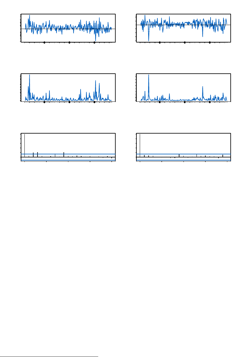
followed by high values. This behavior is conﬁrmed in Figure 2 which shows the

sample autocorrelations of the six series. The log returns show no evidence of serial

correlation, but the squared and absolute returns are positively autocorrelated. Also,

the decay rates of the sample autocorrelations of r

and |r

| appear much slower,

especially for the S&P 500 index, than the exponential rate of a covariance station-

ary autoregressive-moving average (ARMA) process suggesting possible long memory

behavior. Monthly returns, deﬁned as the sum of daily returns over the month, are

illustrated in Figure 3. The monthly returns display much less volatility clustering

than the daily returns.

Table 1 giv es some standard summary statistics along with the Jarque-Bera test

for normality. The latter is computed as

JB =

[

skew

(

kurt −3)

, (1)

where

[

skew denotes the sample skewness and

kurt denotes the sample kurtosis. Under

the null that the data are iid normal, JB is asymptotically distributed as chi-square

∗

The paper was prepared for the Handbook of Financial Time S eries , edited by T.G. Ande rsen ,

R.A. Davis, J-P Kreiss, and T. M ikosch. Thanks to Saraswata Chaudhuri, R ichard Davis, Ron

Scho enberg and Jiahui Wang for helpful comments a nd suggestions. Financial support from the

Gary Waterman Distinguished Scholarship is greatly appreciated.

†

Department of Economics, Box 353330, University of Washington. ezivot@u.washington.edu.

All of the examples in the pap er were constructed using S-PLUS 8.0 and S+FinMetrics 2.0. Script

ﬁles for replicating the examples may be downloaded from http://faculty.washington.edu/ezivot.

1986 1990 1994 1998 2002

-0.30 0.10

Microsoft Returns

1986 1990 1994 1998 2002

-0.20 0.05

S & P 500 Returns

1986 1990 1994 1998 2002

0.00 0.08

Microsoft Squared Returns

1986 1990 1994 1998 2002

0.000 0.040

S & P 500 Squared Returns

1986 1990 1994 1998 2002

0.00 0.30

Microsoft Absolute Returns

1986 1990 1994 1998 2002

0.00 0.30

S & P 500 Absolute Returns

Figure 1: Daily returns, squared returns and absolute returns for Microsoft and the

S&P 500 index.

with 2 degrees of freedom. The distribution of daily returns is clearly non-normal

with negative skewness and pronounced excess kurtosis. Part of this non-normality

is caused by some large outliers around the October 1987 stock market crash and

during the bursting of the 2000 tech bubble. However, the distribution of the data

still appears highly non-normal even after the removal of these outliers. Monthly

returns have a distribution that is much closer to the normal than daily returns.

3 The AR CH and GAR CH Model

[33] showed that the serial correlation in squared returns, or conditional heteroskedas-

ticity, can be modeled using an autoregressive conditional heteroskedast icity (ARCH)

modeloftheform

= E

t−1

]+

, (2)



= z

, (3)

= a

+ a



t−1

+ ···+ a



t−p

, (4)

Lag

ACF

0 5 10 15 20

0.0 0.6

Microsoft Returns

Lag

ACF

0 5 10 15 20

0.0 0.6

S&P 500 Returns

Lag

ACF

0 5 10 15 20

0.0 0.6

Microsoft Squared Returns

Lag

ACF

0 5 10 15 20

0.0 0.6

S&P 500 Squared Returns

Lag

ACF

0 5 10 15 20

0.0 0.6

Microsoft Absolute Returns

Lag

ACF

0 5 10 15 20

0.0 0.6

Microsoft Absolute Returns

Figure 2: Sample autocorrelations of r

and |r

| for Microsoft and S&P 500 index.

where E

t−1

[·] represents expectation conditional on information available at time t−1,

and z

is a sequence of iid random variables with mean zero and unit variance. In the

basic A RCH model z

is assumed to be iid standard normal. The restrictions a

> 0

and a

≥ 0(i =1,...,p) are required for σ

> 0. The representation (2) - (4) is

convenient for deriving properties of the model as well as for specifying the likelihood

function for estimation. The equation for σ

can be rewritten as an AR(p) process

for 



= a

+ a



t−1

+ ···+ a



t−p

+ u

, (5)

where u

= 

−σ

is a martingale diﬀerence sequence (MDS) since E

t−1

]=0and

it is assumed that E(

) < ∞.Ifa

+ ···+ a

< 1 then 

is covariance stationary,

the persistence of 

and σ

is measured by a

+ ···+ a

and ¯σ

=var(

)=E(

/(1 − a

− ···− a

An important extension of the ARCH model proposed by [12] replaces the AR(p)

representation in (4) with an ARMA(p, q) formulation

= a

i=1



t−i

j=1

t−j

, (6)

where the coeﬃcients a

(i =0, ··· ,p) and b

(j =1, ··· ,q) are all assumed to be

1986 1990 1994 1998 2002

-0.3 0.4

Microsoft Returns

1986 1990 1994 1998 2002

-0.20 0.10

S&P 500 Returns

1986 1990 1994 1998 2002

0.02 0.18

Microsoft Squared Returns

1986 1990 1994 1998 2002

0.005

S&P 500 Squared Returns

Lag

ACF

0 5 10 15 20

0.0 0.6

Microsoft Squared Returns

Lag

ACF

0 5 10 15 20

0.0 0.6

S&P 500 Squared Returns

Figure 3: Monthly Returns, Squared Returns and Sample Autocorrelations of

Squared Returns for Microsoft and the S&P 500.

positive to ensure that the conditional variance σ

is always positive.

The model in

(6) together with (2)-(3) is known as the generalized ARCH or GARCH(p, q) model.

The GARCH(p, q) model can be shown to be equivalent to a particular ARCH(∞)

model. When q =0, the GAR CH model reduces to the ARC H model. In order for

the GARCH parameters, b

(j =1, ··· ,q), to be identiﬁed at least one of the ARCH

coeﬃcients a

(i>0) must be nonzero. Usually a GARCH(1,1) model with only

three parameters in the conditional variance equation is adequate to obtain a good

model ﬁtforﬁnancial time series. Indeed, [49] provided compelling evidence that is

diﬃcult to ﬁnd a volatility model that outperforms the simple GARCH(1,1).

Just as an AR CH model can be expressed as an AR model of squared residuals, a

GARCHmodelcanbeexpressedasanARMAmodelofsquaredresiduals.Consider

the GARCH(1,1) model

= a

+ a



t−1

+ b

t−1

. (7)

Since E

t−1

(

)=σ

, (7) can be rewritten as



= a

+(a

+ b

)

t−1

+ u

− b

t−1

, (8)

Positive coeﬃcients are suﬃcient but not necessary conditions for the positivity of c onditional

variance. See [72] and [23] for more general conditions.

whichisanARMA(1,1)modelwithu

= 

− E

t−1

(

) being the MDS disturbance

term.

Given the ARMA(1,1) representation of the GARCH(1,1) model, many of its

properties follow easily from those of the corresponding ARMA(1,1) process for 

For example, the persistence of σ

is captured by a

+ b

and covariance stationarit y

requires that a

+ b

< 1. The cova riance stationary GARCH(1,1) model has an

AR CH(∞) representation with a

= a

i−1

, and the unconditional variance of 

¯σ

= a

/(1 −a

− b

For the general GARCH(p, q) model (6), the squared residuals 

behave like an

ARMA(max(p, q),q) process. Covariance stationarity requires

i=1

j=1

< 1

and the unconditional variance of 

¯σ

=var(

1 −

i=1

j=1

. (9)

3.1 Conditional Mean Speciﬁcation

Depending on the frequency of the data and the type of asset, the conditional mean

t−1

] is typically speciﬁed as a constant or possibly a low order autoregressive-

moving average (ARMA) process to capture autocorrelation caused by market mi-

crostructure eﬀects (e.g., bid-ask bounce) or non-trading eﬀects. If extreme or un-

usual market ev ents have happened during sample period, then dummy variables

associated with these events are often added to th e conditional mean speciﬁcation to

remove these eﬀects. Therefore, the typical conditional mean speciﬁcation is of the

form

t−1

]=c +

i=1

t−i

j=1



t−j

l=0

t−l

+ 

, (10)

where x

is a k × 1 vector of exogenous explanatory variables.

In ﬁnancial investmen t, high risk is often expected to lead to high returns. Al-

though modern capital asset pricing theory does not imply such a simple relationship,

it does suggest that there are some interactions between expected returns and risk as

measured by volatility. Engle, Lilien and Robins (1987) proposed to extend the basic

GARCH model so that the conditional volatility can generate a risk premium which

is part of the expected returns. This extended GARCH model is often referred to

as GARCH-in-the-mean or GARCH-M model. The GARCH-M model extends the

conditional mean equation (10) to include the additional regressor g(σ

),whichcan

be an arbitrary function of conditional volatility σ

. The most common speciﬁcations

are g(σ

)=σ

,σ

, or ln(σ

3.2 Ex planat ory Variables in the Co nditional Var iance Equat io n

Just as exogenous variables may be added to the conditional mean equation, exoge-

nous explanatory variables may also be added to the conditional variance formula (6)

in a straightforward w ay giving

= a

i=1



t−i

j=1

t−j

k=1

t−k

where z

is a m × 1 vector of variables, and δ is a m × 1 vector of positive coeﬃ-

cients. Variables that have been shown to help predict volatility are trading volume,

macroeconomic news announcements ([58], [43], [17]), implied volatility from option

prices and realized volatility ([82], [11]), overnight returns ([46], [68]), and after hours

realized volatility ([21])

3.3 The GARCH M odel and Stylized Facts of Asset Returns

Previously it was shown that the daily returns on Microsoft and the S&P 500 ex-

hibited the “stylized facts” of volatility clustering as w ell as a non-normal empirical

distribution. Researchers have documented these and many other st ylized facts about

the volatility of economic and ﬁnancial time series. [14] gave a complete account of

these facts. Using the ARMA representation of GARCH models shows that the

GARCH model is capable of exp laining many of those stylized facts. The four most

important ones are: volatility clustering, fat tails, volatility mean reversion, and

asymmetry.

To understand volatility clustering, consider the GARCH(1, 1) model in (7). Usu-

ally the GARCH coeﬃcient b

is found to be around 0.9 for many daily or weekly

ﬁnancial time series. Giv en this value of b

,itisobviousthatlargevaluesofσ

t−1

will

be followed b y large values of σ

, and small values of σ

t−1

will be followed b y small

values of σ

. The same reasoning can be obtained from the ARMA represent ation in

(8), where large/small changes in 

t−1

will be followed by large/small changes in 

It is well know n that the distribution of many high frequency ﬁnancial time series

usually have fatter tails than a normal distribution. That is, extreme values occur

more often than implied by a normal distribution. [12] gave the condition for the

existence of the fourth order moment of a GARCH(1, 1) process. Assuming the

fourth order moment exists, [12] showed that the kurtosis implied by a GARCH(1, 1)

process with normal errors is greater than 3, the kurtosis of a normal distribution.

[51] and [52] extended these results to general GARC H(p, q) models. Thus a GARCH

model with normal errors can replicate some of the fat-tailed behavior observed in

ﬁnancial time series. A more thorough discussion of extreme value theory for GARCH

is given by [24]. Most often a GARCH model with a non-normal error distribution

is required to fully capture the observed fat-tailed behavior in returns. These models

are reviewed in sub-Section 6.2.

Although ﬁnancial markets may experience excessive volatilit y from time to time,

it appears that volatilit y will ev entually settle down to a long run level. Recall, the

unconditional variance of 

for the stationary GARCH(1, 1) model is ¯σ

= a

/(1 −

−b

). To see that the volatilit y is always pulled toward this long run, the ARMA

representation in (8) may be rewritten in mean-adjusted form as:

(

− ¯σ

)=(a

+ b

)(

t−1

− ¯σ

)+u

− b

t−1

. (11)

If the abo ve equation is iterated k times, it follows that

(

t+k

− ¯σ

)=(a

+ b

)

(

− ¯σ

)+η

t+k

where η

is a moving average process. Since a

+ b

< 1 for a covariance stationary

GAR CH (1, 1) model, (a

+ b

)

→ 0 as k →∞. Although at time t there may be a

large deviation between 

and the long run variance, 

t+k

− ¯σ

will approach zero

“on average” as k gets large; i.e., the vo latility “mean reverts” to its long run level

¯σ

. The magnitude of a

+ b

controls the speed of mean reversion. The so-called

half-life of a volatility shock, deﬁned as ln(0.5)/ ln(a

+ b

), measures the average

time it takes for |

− ¯σ

| to decrease by one half. Obviously, the closer a

+ b

is to

one the longer is the half-life of a volatility shock. If a

+ b

> 1, the GARCH model

is non-stationary and the volatility will eventually explode to inﬁnit y as k →∞.

Similar arguments can be easily constructed for a GARCH(p, q) model.

The standard GARCH(p, q) model with Gaussian errors implies a symmetric dis-

tribution for y

and so cannot account for the observed asymmetry in the distribution

of returns. Ho wever, as shown in Section 6, asymmetry can easily be built into the

GARCH model by allowing 

to have an asymmetric distribution or by explicitly

modeling asymmetric behavior in the conditional variance equation (6).

3.4 Temporal Aggregation

Volatility clustering and non-Gaussian behavior in ﬁnancial returns is typically seen

in weekly, daily or intraday data. The persistence of conditional volatility tends to

increase with the sampling frequency

. However, as shown in [32], for GARCH models

there is no simple aggregation principle that links the parameters of the model at

one sampling frequency to the parameters at another frequency. This occurs because

GAR C H models imply that the squared residual process follows an ARMA t ype

process with MDS innovations which is not closed under temporal aggregation. The

practical result is that GARCH models tend to be ﬁt to the frequency at hand. This

strategy, however, may not provide the best out-of-sample volatility forecasts. For

example, [68] showed that a GARCH model ﬁt to S&P 500 daily returns produces

better forecasts of weekly and month ly volatility than GARCH models ﬁttoweekly

or monthly returns, respectively.

4 T esting for ARCH/GARCH eﬀects

The stylized fact of volatility clustering in returns manifests itself as autocorrelation

in squared and absolute returns or in the residuals from the estimated conditional

mean equation (10). The signiﬁcance of these autocorrelations may be tested using

The empirical result that aggregated returns exhib it sm aller GARCH e ﬀects and approach

Gaussian behavior can be explained by the results of [26] who showed that a central limit the-

orem holds for standardized sums of random variables that follow covariance stationary GARCH

pro cesses.

the Ljung-Box or modiﬁed Q-statistic

MQ(p)=T (T +2)

j=1

ˆρ

T − j

, (12)

where ˆρ

denotes the j-lag sample autocorrelation of the squared or absolute returns.

IfthedataarewhitenoisethentheMQ(p) statistic has an asymptotic chi-square dis-

tribution with p degrees of freedom. A signiﬁcant value for MQ(p) provides evidence

for time varying conditional volatility.

To test for autocorrelation in the raw returns when it is suspected that there are

GAR CH eﬀects present, [27] suggested using the following heteroskedasticity robust

version of (12)

(p)=T(T +2)

j=1

T − j

ˆσ

+ˆγ

ˆρ

where ˆσ

is a consisten t estimate of the squared unconditional variance of returns,

and ˆγ

is the sample autocovariance of squared returns.

Since an ARCH model implies an AR model for the squared residuals 

, [33]

showed that a simple Lagrange multiplier (LM) test for ARCH eﬀects can be con-

structed based on the auxiliary regression (5). Under the null hypothesis that there

are no A RCH eﬀects, a

= a

= ···= a

=0, the test statistic

LM = T · R

(13)

has an asymptotic chi-square distribution with p degrees of freedom, where T is the

sample size and R

is computed from the regression (5) using estimated residuals.

Even though the LM test is constructed from an ARCH model, [61] show that it

also has power against more general GARCH alternatives and so it can be used as a

general speciﬁcation test for GARCH eﬀects.

[64], however, argued that the LM test (13) may reject if there is general mis-

speciﬁcation in the conditional mean equation (10). They showed that such misspec-

iﬁcation causes the estimated residuals ˆ

to be serially correlated which, in turn,

causes ˆ

to be serially correlated. Therefore, care should be exercised in specifying

the conditional mean equation (10) prior to testing for AR CH eﬀects.

4.1 Testing for ARCH Eﬀects in Daily and M onthly R etur ns

Table 2 shows values of MQ(p) computed from daily and monthly squared returns

and the LM test for ARCH, for various values of p, for Microsoft and the S&P 500.

There is clear evide n ce of volatility clustering in the daily returns, but less evidence

for monthly returns especially for the S&P 500.

5 Estimation of GA RCH M odels

The general GARCH(p, q) model with normal errors is (2), (3) and (6) with z

∼

iid N(0, 1). For simplicity, assume that E

t−1

]=c. Given that 

follows Gaussian

MQ(p) r

Asset p 15101510

Daily Returns

MSFT

56.81

(0.000)

562.1

(0.000)

206.8

(0.000)

56.76

(0.000)

377.9

(0.000)

416.6

(0.000)

S&P 500

87.59

(0.000)

415.5

(0.000)

456.1

(0.000)

87.52

(0.000)

311.4

(0.000)

329.8

(0.000)

Monthly Returns

MSFT

0.463

(0.496)

17.48

(0.003)

31.59

(0.000)

0.455

(0.496)

16.74

(0.005)

33.34

(0.000)

S&P 500

1.296

(0.255)

2.590

(0.763)

6.344

(0.786)

1.273

(0.259)

2.229

(0.817)

5.931

(0.821)

Notes: p-values are in parentheses.

Table 2: Tests for ARCH Eﬀects in Daily Stock Returns

distribution conditional on past history, the prediction error decomposition of the

log-likelihood function of the GARCH model conditional on initial values is

log L =

t=1

= −

log(2π) −

t=1

log σ

−

t=1



, (14)

where l

= −

(log(2π)+logσ

) −



. The conditional loglikelihood (14) is used

in practice since the unconditional distribution of the initial values is not known

in closed form

. As discussed in [69] and [20], there are several practical issues to

consider in the maximization of (14). Starting values for the model parameters c, a

(i =0, ··· ,p) and b

(j =1, ··· ,q) need to be chosen and an initialization of 

and

must be supplied. The sample mean of y

is usually used as the starting value for

c, zero values are often given for the conditional variance parameters other than a

and a

, and a

is set equal to the unconditional variance o f y

. For the initial values

of σ

, a popular choice is

= 

s=1



,t≤ 0,

where the initial values for 

are computed as the residuals from a regression of y

on a constant.

Once the log-likelihood is initialized, it can be maximized using numerical op-

timization techniques. The most common method is based on a Newton-Raphson

iteration of the form

n+1

− λ

)

−1

[29] gave a computationally intensive numerical pro cedure for approximating the exact log-

likelihood.

Setting the starting values for all of the A RCH coeﬃcients a

(i =1,...,p) to ze ro may create

an ill-behaved likelihood and lead to a local minimum since the remaining GARCH parameters are

not identiﬁed.

where θ

denotes the vector of estimated model parameters at iteration n, λ

is a

scalar step-length parameter, and s(θ

) and H(θ

) denote the gradien t (or score)

vector and Hessian matrix of the log-likelihood at iteration n, respectively. The step

length parameter λ

is chosen such that ln L(θ

n+1

) ≥ ln L(θ

). For GARCH models,

the BHHH algorithm is often used. This algorithm approximates the Hessian matrix

using only ﬁrst derivative information

−H(θ) ≈ B(θ)=

t=1

∂l

∂θ

∂l

∂θ

In the application of the Newton-Raphson algorithm, analytic or numerical deriva-

tives may be used. [41] pro vided algorithms for computing analytic derivatives for

GARCH models.

The estimates that maximize the conditional log-likelihood (14) are called the

maximum likelihood (ML) estimates. Under suitable regularity conditions, the ML

estimates are consistent and asymptotically normally distributed and an estimate of

the asymptotic covariance matrix of the ML estimates is constructed from an estimate

of the ﬁnal Hessian matrix from the optimization algorithm used. Unfortunately,

veriﬁcation of the appropriate regularity conditions has only been done for a limited

number of simple GARCH models, see [63], [60], [55], [56] and [81]. In practice, it is

generally assumed that the necessary regularity conditions are satisﬁed.

In GARCH models for which the distribution of z

is symmetric and the parame-

ters of the conditional mean and variance equations are variation free, the information

matrix of the log-lik elihood is block diagonal. The implication of this is that the pa-

rameters of the conditional mean equation can be estimated separately from those

of the conditional variance equation without loss of asymptotic eﬃciency. This can

greatly simplify estimation. An common model for which block diagonality of the

information matrix fails is the GARCH-M model.

5.1 Num erical Accuracy of GARCH Estimates

GARCH estimation is widely available in a number of commercial software packages

(e.g. EVIEWS, GAUSS, MATLAB, Ox, RATS, S-PLUS, TSP) and there are also

a few free open source implementations. [41], [69], and [20] discussed numerical ac-

curacy issues associated with maximizing the GARCH log-likelihood. They found

that starting values, optimization algorithm choice, and use of analytic or numerical

derivatives, and convergence criteria all inﬂuence the resulting numerical estimates

of the GARCH parameters. [69] and [20] studied estimation of a GARCH(1,1) model

from a variety of commercial statistical packages using the exchange rate data of [15]

as a benchmark. They found that it is often diﬃcult to compare competing software

since the exact construction of the GAR CH likelihood is not always adequately de-

scribed. In general, they found that use of analytic derivatives leads to more accurate

estimation than procedures based on purely numerical evaluations.

In practice, the GARCH log-likelihood function is not always well behaved, es-

pecially in complicated models with many parameters, and reaching a global max-

imum of the log-likelihood function is not guaranteed using standard optimization

techniques. Also, the positive variance and stationarity constraints are not straight-

forward to implement with common optimization software and are often ignored in

practice. P oor choice of starting values can lead to an ill-behaved log-likelihood and

cause convergence problems. Therefore, it is always a good idea to explore the surface

of the log-likelihood by perturbing the starting values and re-estimating the GARC H

parameters.

In many empirical applications of the GARCH(1,1) model, the estimate of a

isclosetozeroandtheestimateofb

is close to unity. This situation is of some

concern since the GARCH parameter b

becomes unidentiﬁed if a

=0, and it is

well kno w n that the distribution of ML estimates can become ill-behaved in models

with nearly unidentiﬁed parameters. [66] studied the accuracy of ML estimates of

the GARCH parameters a

and b

when a

is close to zero. They found that the

estimated standard error for b

is spuriously small and that the t-statistics for testing

hypotheses about the true value of b

are severely size distorted. They also showed

that the concentrated loglikelihood as a function of b

exhibits multiple maxima. To

guard against spurious inference they recommended comparing estimates from pure

AR CH(p) models, which do not suﬀer from the identiﬁcation problem, with estimates

from the GARCH(1,1). If the volatility dynamics from these models are similar then

the spurious inference problem is not likely to be present.

5.2 Quasi-M axim um Likelihood Estimation

Another practical issue associated with GARCH estimation concerns the correct

choice of the error distribution. In particular, the assumption of conditional normality

is not always appropriate. However, as shown by [86] and [16], even when normal-

ity is inappropriately assumed, maximizing the Gaussian log-likelihood (14) results

in quasi-maximum likelihood estimates (QMLEs) that are consistent and asymptot-

ically normally distributed provided the conditional mean and variance functions of

the GAR CH model are correctly speciﬁed. Inaddition,[16]derivedanasymptotic

covariance matrix for the QMLEs that is robust to conditional non-normality. This

matrix is estimated using

QML

)

−1

QML

)H(

QML

)

−1

, (15)

where

QML

denotes the QMLE of θ, and is often called the “sandwich” estima-

tor. The coeﬃcient standard errors computed from the square roots of the diagonal

elements of (15) are sometimes called “Bollerslev-Wooldridge” standard errors. Of

course, the QMLEs will be less eﬃcient than the true MLEs based on the correct er-

ror distribution. However, if the normality assumption is correct then the sandwich

covariance is asymptotically equivalent to the inverse of the Hessian. As a result, it

is good practice to routinely use t h e sandwich covariance for inference purposes.

[35] and [16] evaluated the accuracy of the quasi-maximum likelihood estimation

of GARCH(1,1) models. They found that if the distribution of z

in (3) is symmetric,

then QMLE is often close to the MLE. However, if z

has a skewed distribution then

theQMLEcanbequitediﬀerent from the MLE.

5.3 Model Selectio n

An important practical problem is the determination of the ARCH order p and the

GARCH order q for a particular series. Since GARCH models can be treated as

ARMA models for squared residuals, traditional model selection criteria such as the

Akaike information criterion (AIC) and the Bayesian information criterion (BIC) can

be used for selecting models. For daily returns, if attention is restricted to pure

AR CH(p) models it is typically found that large values of p are selected b y AIC and

BIC. For GARCH(p, q) models, those with p, q ≤ 2 are typically selected by AIC

and BIC. Lo w order GARCH(p,q) models are generally preferred to a high order

AR CH(p) for reasons of parsimon y and better numerical stability of estimation (high

order GARCH(p, q) processes often have many local maxima and minima). For many

applications, it is hard to beat the simple GARC H(1,1) model.

5.4 Evaluat io n of Es timated GARCH models

After a GARCH model has been ﬁt to the data, the adequacy of the ﬁtcanbe

evaluated using a number of graphical and statistical diagnostics. If the GARCH

model is correctly speciﬁed, then the estimated standardized residuals ˆ

/ˆσ

should

behave like classical regression residuals; i.e., they should not display serial correla-

tion, conditional heteroskedasticity or any type of nonlinear dependence. In addition,

the distribution of the standardized residuals ˆ

/ˆσ

should match the speciﬁed error

distribution used in the estimation.

Graphically, ARCH eﬀects reﬂected by serial correlation in ˆ

/ˆσ

can be uncovered

by plotting its SACF. The modiﬁed Ljung-Box statistic (12) can be used to test the

null of no autocorrelation up to a speciﬁc lag, and Engle’s LM statistic (13) can be

used to test the null of no remaining ARCH eﬀects

. If it is assumed that the errors

are Gaussian, then a plot of ˆ

/ˆσ

against time should have roughly ninety ﬁve percent

of its values between ±2; a normal qq-plot of ˆ

/ˆσ

should look roughly linear

;and

the JB statistic should not be too mu ch larger than six.

5.5 Estima tio n of GA RCH Models for D a ily and M o nthly R etu rn s

Table 3 gives model selection criteria for a variety of GARCH(p, q) ﬁtted to the daily

returns on Microsoft and the S&P 500. For pure ARC H(p) models, an ARCH(5)

is chosen by all criteria for both series. For GARCH(p, q) models, AIC picks a

GARCH(2,1) for both series and BIC picks a GARCH(1,1) for both series

Table4givesQMLEsoftheGARCH(1,1)model assuming normal errors for the

Microsoft and S&P 500 daily returns. For both series, the estimates of a

are around

These tests should be viewed as ind icative, since the distribution of the tests a re inﬂuenced by

the estimation of the GARCH model. For valid LM tests, the partial derivatives of σ

with respect

to the conditional volatility parameters should b e added as additional regressors in the auxiliary

regression (5) based on estimated residuals.

If an error distribution other than the Gaussian is assumed, then the qq-plot should be con-

structed using the quantiles of the assumed distribution.

The low log-likelihood values for the GARCH(2,2) models indicate that a local maximum was

reached.

(p, q) Asset AIC BIC Likelihood

(1,0) MSFT -19977 -19958 9992

S&P 500 -27337 -27318 13671

(2,0) MSFT -20086 -20060 10047

S&P 500 -27584 -27558 13796

(3,0) MSFT -20175 -20143 10092

S&P 500 -27713 -27681 13861

(4,0) MSFT -20196 -20158 10104

S&P 500 -27883 -27845 13947

(5,0) MSFT -20211 -20166 10113

S&P 500 -27932 -27887 13973

(1,1) MSFT -20290 -20264 10149

S&P 500 -28134 -28109 14071

(1,2) MSFT -20290 -20258 10150

S&P 500 -28135 -28103 14072

(2,1) MSFT -20292 -20260 10151

S&P 500 -28140 -28108 14075

(2,2) MSFT -20288 -20249 10150

S&P 500 -27858 -27820 13935

Table 3: Model Selection Criteria for Estimated GARCH(p,q) Models.

0.09 and the estimates of b

are around 0.9. Using both ML and QML standard er-

rors, these estimates are statistically diﬀerent from zero. Howev er, the QML standard

errors are considerably larger than the ML standard errors. The estimated volatility

persistence, a

+ b

, is very high for both series and implies half-lives of shocks to

volatility to Microsoft and the S&P 500 of 15.5 days and 76 days, respectively. The

unconditional standard deviation of returns, ¯σ =

/(1 − a

− b

), for Microsoft

and the S&P 500 implied by the GARCH(1,1) models are 0.0253 and 0.0138, respec-

tively, and are very close to the sample standard deviations of returns reported in

Table 1.

Estimates of GARCH-M(1,1) models for Microsoft and the S&P 500, where σ

is added as a regressor to the mean equation, show small positive coeﬃcients on σ

and essentially the same estimates for the remaining parameters as the GARCH(1,1)

models.

Figure 4 shows the ﬁrst diﬀerences of returns along with the ﬁtted one-step-

ahead volatilities, ˆσ

, computed from the GARCH(1,1) and ARCH(5) models. The

ARCH(5) and GARCH(1,1) models do a good job of capturing the observed volatil-

ity clustering in returns. The GARCH(1,1) volatilities, however, are smoother and

display more persistence than the ARC H(5) volatilities.

Graphical diagnostics from the ﬁtted GARCH(1,1) models are illustrated in Fig-

ure 5. The SACF of ˆ

/ˆσ

does not indicate any signiﬁcant autocorrelation, but

the normal qq-plot of ˆ

/ˆσ

shows strong departures from normality. The last three

columns of Table 4 give the standard statistical diagnostics of the ﬁtted GARCH

GARCH Parameters Residual Diagnostics

Asset a

MQ(12) LM(12) JB

Daily Returns

MSFT

2.80e

−5

(3.42e

−6

)

[1.10e

−5

]

0.0904

(0.0059)

[0.0245]

0.8658

(0.0102)

[0.0371]

4.787

(0.965)

4.764

(0.965)

1751

(0.000)

S&P 500

1.72e

−6

(2.00e

−7

)

[1.25e

−6

]

0.0919

(0.0029)

[0.0041]

0.8990

(0.0046)

[0.0436]

5.154

(0.953)

5.082

(0.955)

5067

(0.000)

Monthly Returns

MSFT

0.0006

[0.0006]

0.1004

[0.0614]

0.8525

[0.0869]

8.649

(0.733)

6.643

(0.880)

3.587

(0.167)

S&P 500

3.7e

−5

[9.6e

−5

]

0.0675

[0.0248]

0.9179

[0.0490]

3.594

(0.000)

3.660

(0.988)

72.05

(0.000)

Notes: QML standard errors are in brackets.

Table 4: Estimates of GARCH(1,1) Model with Diagnostics.

models. Consistent with the SACF, the MQ statistic and Engle’s LM statistic do

not indicate remain ing ARCH eﬀects. Furthermore, the extremely large JB statistic

conﬁrms nonnormality.

Table 4 also sho ws estimates of GARCH(1,1) models ﬁt to the monthly returns.

The GARCH(1,1) models ﬁt to the monthly returns are remarkable similar to those

ﬁt to the daily returns. There are, however, some important diﬀerences. The monthly

standardized residuals are much closer to the normal distribution, especially for Mi-

crosoft. Also, the GARCH estimates for the S&P 500 reﬂect some of the character-

istics of spurious GARCH eﬀects as discussed in [66]. In particular, the estimate of

is close to zero, and has a relatively large QML standard error, and the estimate

of b

is close to one and has a very small standard error.

6GARCHModelExtensions

In many cases, the basic GARCH conditional variance equation (6) under normality

provides a reasonably good model for analyzing ﬁnancial time series and estimating

conditional volatility. Howev er, in some cases there are aspects of the model which

can be improved so that it can better capture the characteristics and dynamics of a

particular time series. For example, the empirical analysis in the previous Section

showed that for the daily returns on Microsoft and the S&P 500, the normality

assumption may not be appropriate and there is evidence of nonlinear behavior in

the standardized residuals from the ﬁtted GARCH(1,1) model. This Section discusses

several extensions to the basic GARCH model that make GARCH modeling more

ﬂexible.

1986 1990 1994 1998 2002

-0.30 0.10

Microsoft Daily Returns

1986 1990 1994 1998 2002

-0.20 0.05

S&P 500 Daily Returns

1986 1990 1994 1998 2002

0.02 0.10

Conditional Volatility from GARCH(1,1)

1986 1990 1994 1998 2002

0.01 0.06

Conditional Volatility from GARCH(1,1)

1986 1990 1994 1998 2002

0.02 0.10

Conditional Volatility from ARCH(5)

1986 1990 1994 1998 2002

0.01 0.09

Conditional Volatility from ARCH(5)

Figure 4: One-step ahead volatilities from ﬁtted ARCH(5) and GARCH(1,1) models

for Microsoft and S&P 500 index.

6.1 Asym metric Leverage Eﬀects and News Impact

In the basic GARCH model (6), since only squared residuals 

t−i

enter the conditional

variance equation, the signs of the residuals or shocks have no eﬀect on conditional

volatility. However, a stylized fact of ﬁnancial volatility is that bad news (negative

shocks) tends to have a larger impact on volatility than good news (positiv e shock s).

That is, volatilit y tends to be higher in a falling market than in a rising market. [10]

attributed this eﬀect to the fact that bad news tends to drive down the stock price,

thus increasing the leverage (i.e., the debt-equity ratio) of the stock and causing the

stock to be more volatile. Based on this conjecture, the asymmetric news impact on

volatilit y is commonly referred to as the leverage eﬀect.

6.1.1 Testing for Asymmetric Eﬀects on Conditional Volatility

A simple diagnostic for uncovering possible asymmetric leverage eﬀectsisthesample

correlation between r

and r

t−1

. A negative value of this correlation provides some

evidence for potential leverage eﬀects. Other simple diagnostics, suggested by [39],

Lag

ACF

0 102030

0.0 0.4 0.8

Microsoft Squared Residuals

Lag

ACF

0102030

0.0 0.4 0.8

S&P 500 Squared Residuals

Quantiles of Standard Normal

Microsoft Standardized Residuals

-2 0 2

-0.3 -0.1 0.1

Quantiles of Standard Normal

S&P 500 Standardized Residuals

-2 0 2

-0.20 -0.05 0.10

Figure 5: Graphical residual diagnostics from ﬁtted GARCH(1,1) models to Microsoft

and S&P 500 returns.

result from estimating the following test regression

ˆε

= β

+ β

ˆw

t−1

+ ξ

where ˆε

is the estimated residual from the conditional mean equation (10), and ˆw

t−1

is a variable constructed from ˆε

t−1

and the sign of ˆε

t−1

. Asigniﬁcant value of β

indicates evidence for asymmetric eﬀects on conditional volatility. Let S

−

t−1

denote

a dummy variable equal to unity when ˆε

t−1

is negative, and zero otherwi se. Engle

and Ng consider three tests for asymmetry. Setting ˆw

t−1

= S

−

t−1

gives the Sign

Bias test; setting ˆw

t−1

= S

−

t−1

ˆε

t−1

gives the Negative Size Bias test; and setting

ˆw

t−1

= S

t−1

ˆε

t−1

gives the Positive Size Bias test.

6.1.2 Asymmetric GARCH Models

The leverage eﬀect can be incorporated into a GARCH model in several ways. [71]

proposed the following exponen tial GARCH (EGARCH) model to allow for leverage

eﬀects

= a

i=1

|

t−i

| + γ



t−i

j=1

t−j

, (16)

where h

=logσ

.Notethatwhen

t−i

is positive or there is “good news”, the

total eﬀect of 

t−i

is (1 + γ

)|

t−i

|; in contrast, when 

t−i

is negative or there is “bad

news”, the total eﬀect of 

t−i

is (1 − γ

)|

t−i

|. Bad news can have a larger impact on

volatility, and the value of γ

would be expected to be negative. An advantage of the

EGARCH model over the basic GARCH model is that the conditional variance σ

guaranteed to be positive regardless of the values of the coeﬃcients in (16), because

the logarithm of σ

instead of σ

itself is modeled. Also, the EGARCH is covariance

stationary provided

j=1

< 1.

Another GARCH variant that is capable of modeling leverage eﬀectsisthethresh-

old GARCH (TGARCH) model,

which has the following form

= a

i=1



t−i

i=1

t−i



t−i

j=1

t−j

, (17)

where

t−i

1if

t−i

< 0

0if

t−i

≥ 0

That is, depending on whether 

t−i

is above or below the threshold value of zero,



t−i

has diﬀerent eﬀects on the conditional variance σ

:when

t−i

is positive, the

total eﬀects are given by a



t−i

;when

t−i

is negative, the total eﬀects are given by

+ γ

)

t−i

. So one would expect γ

to be positive for bad news to have larger

impacts.

[31] extended the basic GARCH model to allow for leverage eﬀects. Their power

GAR CH (PGARCH(p, d, q)) model has the form

= a

i=1

(|

t−i

| + γ



t−i

)

j=1

t−j

, (18)

where d is a positiv e exponent, and γ

denotes the coeﬃcient of leverage eﬀects.

When d =2, (18) reduces to the basic GARCH model with leverage eﬀects. When

d =1, the PGARCH model is speciﬁed in terms of σ

which tends to be less sensitive

to outliers than when d =2. The exponent d may also be estimated as an additional

parameter which increases the ﬂexibility of the model. [31] sho wed that the PGARCH

model also includes man y other GARCH variants as special cases.

Many other asymmetric GARCH models have been proposed based on smooth

transition and Markov switching models. See [44] and [83] for excellent surveys of

these models.

6.1.3 News Impact Curve

The GAR CH, EGARC H, TGARCH and PGARCH models are all capable of modeling

leverage eﬀect s. To clearly see the impact of leverage eﬀects in these models, [75],

and [39] advocated the use of the so-called news impact curve. They deﬁned the news

The original TGARCH mo del prop osed by [87] models σ

instead of σ

. The TGARCH model

is also known as the GJR m odel because [47] proposed essentially the same m odel.

GAR CH(1, 1) σ

= A + a

(|

t−1

| + γ



t−1

)

A = a

+ b

¯σ

= a

/[1 − a

(1 + γ

) − b

]

TGARCH(1, 1) σ

= A +(a

+ γ

t−1

)

t−1

A = a

+ b

¯σ

= a

/[1 − (a

+ γ

/2) − b

]

PGAR CH(1, 1, 1) σ

= A +2

√

(|

t−1

| + γ



t−1

)

(|

t−1

| + γ



t−1

)

, A =(a

+ b

¯σ)

¯σ

= a

/[1 − a

2/π − b

]

EGAR CH(1, 1) σ

= A exp{a

(|

t−1

| + γ



t−1

)/¯σ}

A =¯σ

exp{a

}

¯σ

=exp{(a

+ a

2/π)/(1 − b

)}

Table 5: News impact curves for asymmetric GARCH processes. ¯σ

denotes the

unconditional variance.

Asset corr(r

t−1

) Sign Bias Negative Size Bias Positive Size Bias

Microsoft −0.0315

−0.4417

(0.6587)

−6.816

(0.000)

3.174

(0.001)

S&P 500 −0.098

2.457

(0.014)

−11.185

(0.000)

1.356

(0.175)

Notes: p-values are in parentheses.

Table 6: Tests for Asymmetric GARCH Eﬀects.

impact curve as the functional relationship between conditional variance at time t

and the shock term (error term) at time t−1, holding constant the information dated

t−2 and earlier, and with all lagged conditional variance evaluated at the level of the

unconditional variance. Table 5 summarizes the expressions deﬁning the news impact

curves, which include expressions for the unconditional variances, for the asymmetric

GARCH(1,1) models.

6.1.4 Asymmetric GARCH Models for Daily Returns

Table 6 shows diagnostics and tests for asymmetric eﬀects in the daily returns on

Microsoft and the S&P 500. The correlation between r

and r

t−1

is negative and

fairly small for both series indicating weak evidence for asymmetry. However, the

Size Bias tests clearly indicate asymmetric eﬀects with the Negative Size Bias test

giving the most signiﬁcant results.

Table 7 gives the estimation results for EGAR CH(1,1), TGARCH(1,1) and PGARCH(1,d,1)

models for d =1, 2. All of the asymmetric models show statistically signiﬁcant lever-

Model a

BIC

Microsoft

EGARCH

−0.7273

[0.4064]

0.2144

[0.0594]

0.9247

[0.0489]

−0.2417

[0.0758]

-20265

TGAR CH

3.01e

−5

[1.02e

−5

]

0.0564

[0.0141]

0.8581

[0.0342]

0.0771

[0.0306]

-20291

PGARCH 2

2.87e

−5

[9.27e

−6

]

0.0853

[0.0206]

0.8672

[0.0313]

−0.2164

[0.0579]

-20290

PGARCH 1

0.0010

[0.0006]

0.0921

[0.0236]

0.8876

[0.0401]

−0.2397

[0.0813]

-20268

S&P 500

EGARCH

−0.2602

[0.3699]

0.0720

[0.0397]

0.9781

[0.0389]

−0.3985

[0.4607]

-28051

TGAR CH

1.7e

−6

[7.93e

−7

]

0.0157

[0.0081]

0.9169

[0.0239]

0.1056

0.0357

-28200

PGARCH 2

1.78e

−6

[8.74e

−7

]

0.0578

[0.0165]

0.9138

[0.0253]

−0.4783

[0.0910]

-28202

PGARCH 1

0.0002

[2.56e

−6

]

0.0723

[0.0003]

0.9251

[8.26e

−6

]

−0.7290

[0.0020]

-28253

Notes: QML standard errors are in brac kets.

Table 7: Estimates of Asymmetric GARCH(1,1) Models.

age eﬀects, and lower BIC values than the symmetric GARCH models. Model selec-

tion criteria indicate that the TGARCH(1,1) is the best ﬁtting model for Microsoft,

and the PGARCH(1,1,1) is the best ﬁtting model for the S&P 500.

Figure 6 shows the estimated news impact curves based on these models. In

this plot, the range of 

is determined by the residuals from the ﬁtted models. The

TGARCH and PGARCH(1,2,1) models ha ve very similar NICs and show much larger

responses to negative shocks than to positive shocks. Since the EGARCH(1,1) and

PGARCH(1,1,1) models are more robust to extreme shocks, impacts of small (large)

shocks for these model are larger (smaller) compared to those from the other models

and the leverage eﬀect is less pronounced.

6.2 Non-Gaussian Error Distributions

In all the examples illustrated so far, a normal error distribution has been exclusively

used. However, given the well known fat tails in ﬁnancial time series, it may be more

appropriate to use a distribution which has fatter tails than the normal distribution.

The most common fat-tailed error distributions for ﬁtting GARCH models are: the

Student’s t distribution; the double exponential distribution; and the generalized

error distribution.

[13] proposed ﬁtting a GARCH model with a Student’s t distribution for the

standardized residual. If a random variable u

has a Student’s t distribution with ν

degrees of freedom and a scale parameter s

, the probability density function (pdf)

-0.2 -0.1 0.0 0.1 0.2

0.001 0.004

Asymmetric GARCH(1,1) Models for Microsoft

TGARCH

PGARCH 1

PGARCH 2

EGARCH

-0.2 -0.1 0.0 0.1 0.2

0.0 0.002 0.005

Asymmetric GARCH(1,1) Models for S&P 500

TGARCH

PGARCH 1

PGARCH 2

EGARCH

Figure 6: News impact curves from ﬁtted asymmetric GARC H(1,1) models for Mi-

crosoft and S&P 500 index.

of u

is given by

f(u

Γ[(ν +1)/2]

(πν)

1/2

Γ(ν/2)

−1/2

[1 + u

/(s

ν)]

(ν+1)/2

where Γ(·) is the gamma function. The variance of u

is given by

var(u

ν − 2

,v>2.

If the error term 

in a GARCH model follows a Student’s t distribution with ν

degrees of freedom and var

t−1

(

)=σ

, the scale parameter s

should be chosen to

(ν − 2)

Thus the log-likelihood function of a GARCH model with Student’s t distributed

errors can be easily constructed based on the a bo ve pdf.

[71] proposed to use the generalized error distribution (GED) to capture the fat

tails usually observed in the distribution of ﬁnancial time series. If a random variable

has a GED with mean zero and unit variance, the pdf of u

is given by

f(u

ν exp[−(1/2)|u

/λ|

]

λ · 2

(ν+1)/ν

Γ(1/ν)

where

λ =

−2/ν

Γ(1/ν)

Γ(3/ν)

1/2

and ν is a positive parameter governing the thickness of the tail behavior of the

distribution. When ν =2the above pdf reduces to the standard normal pdf; when

ν<2, the density has thicker tails than the normal density; when ν>2, the density

has thinner tails than the normal density.

When the tail thickness parameter ν =1, the pdf of GED reduces to the pdf of

double exponential distribution:

f(u

√

−

√

2|u

Based on the above pdf, the log-likelihood function of GARCH models with GED or

double exponential distributed errors can be easily constructed. See to [48] for an

example.

Several other non-Gaussian error distribution have been proposed. [42] in troduced

the asymmetric Studen t’s t distribution to capture both skewness and excess kurtosis

in the standardized residuals. [85] proposed the normal inverse Gaussian distribution.

[45] provided a very ﬂexible seminonparametric innovation distribution based on a

Hermite expansion of a Gaussian density. Their expansion is capable of capturing

general shape departures from Gaussian behavior in the standardized residuals of the

GARCH model.

6.2.1 Non-Gaussian GARCH Models for Daily Returns

Table 8 gives estimates of the GARCH(1,1) and best ﬁtting asymmetric GARCH(1,1)

models using Student’s t innovations for the Microsoft and S&P 500 returns. Model

selection criteria indicated that models using the Student’s t distribution ﬁt better

than the models using the GED distribution. The estimated degrees of freedom for

Microsoft is about 7, and for the S&P 500 about 6. The use of t-distributed errors

clearly improves the ﬁt of the GARCH(1,1) models. Indeed, the BIC values are even

lower than the values for the asymmetric GARCH(1,1) models based on Gaussian

errors (see Table 7). Ov erall, the asymmetric GAR CH(1,1) models with t-distributed

errors are the best ﬁtting models. The qq-plots in Figure 7 shows that the Student’s t

distribution adequately captures the fat-tailed behavio r in the standardized residuals

for Microsoft but not for the S&P 500 index.

7 Long Mem ory GARCH Models

If returns follow a GARCH(p, q) model, then the autocorrelations of the squared and

absolute returns should decay exponentially. However, the SACF of r

and |r

| for

Model a

v BIC

Microsoft

GARCH

3.39e

−5

[1.52e

−5

]

0.0939

[0.0241]

0.8506

[0.0468]

6.856

[0.7121

-20504

TGAR CH

3.44e

−5

[1.20e

−5

]

0.0613

[0.0143]

0.8454

[0.0380]

0.0769

[0.0241]

7.070

[0.7023]

-20511

S&P 500

GARCH

5.41e

−7

[2.15e

−7

]

0.0540

[0.0095]

0.0943

[0.0097]

5.677

[0.5571]

-28463

PGAR CH

d =1

0.0001

[0.0002]

0.0624

[0.0459]

0.9408

[0.0564]

−0.7035

[0.0793]

6.214

[0.6369]

-28540

Notes: QML standard errors are in brackets.

Table 8: Estimates of Non Gaussian GARCH(1,1) Models.

Microsoft and the S&P 500 in Figure 2 appear to decay much more slowly. This is

evidence of so-called long memory behavior. Formally, a stationary process has long

memory or long range dependence if its autocorrelation function behaves like

ρ(k) → C

2d−1

as k →∞,

where C

is a positive constant, and d is a real number between 0 and

. Thus the

autocorrelation function of a long memory process decays slowly at a hyperbolic rate.

In fact, it decays so slowly that the autocorrelations are not summable:

∞

k=−∞

ρ(k)=∞.

It is important to note that the scaling property of the autocorrelation function does

not dictate the general behavior of the autocorrelation function. Instead, it only

speciﬁes the asymptotic behavior when k →∞. What this means is that for a long

memory process, it is not necessary for the autocorrelation to remain signiﬁcant at

large lags as long as the autocorrelation function decays slowly. [8] gives an example

to illustrate this property.

The following subSections describe testing for long memory and GARCH models

that can capture long memory behavior in volatility. Explicit long memory GARCH

models are discussed in [83].

7.1 Testing for Long Mem ory

One of the best-known and easiest to use tests for long memory or long range de-

pendence is the rescaled range (R/S) statistic, which was originally proposed by [53],

and later reﬁned by [67] and his coauthors. The R/S statistic is the range of partial

sums of deviations of a time series from its mean, rescaled by its standard deviation.

Speciﬁcally, consider a time series y

,fort =1, ··· ,T. The R/S statistic is deﬁned

-10

-5

-5 0 5

Microsoft

-5 0 5

S&P 500

Figure 7: QQ-plots of Standardized Residuals from Asymmetric GARCH(1,1) models

with Student’s t errors.

⎡

⎣

max

1≤k≤T

j=1

− ¯y) − min

1≤k≤T

j=1

− ¯y)

⎤

⎦

, (19)

where ¯y =1/T

i=1

and s

1/T

i=1

− ¯y)

.Ify

is iid with ﬁnite variance,

then

√

⇒ V,

where ⇒ denotes weak convergence and V is the range of a Brownian bridge on the

unit interval. [62] gives selected quantiles of V .

[62] pointed out that the R/S statistic is not robust to short range dependence. In

particular, if y

is autocorrelated (has short memory) then the limiting distribution

of Q

√

T is V scaledbythesquarerootofthelongrunvarianceofy

. To allow for

short range dependence in y

, [62] modiﬁed the R/S statistic as follows

ˆσ

(q)

⎡

⎣

max

1≤k≤T

j=1

− ¯y) − min

1≤k≤T

j=1

− ¯y)

⎤

⎦

, (20)

where the sample standard deviation is replaced by the square root of the Newey-

West ([73]) estimate of the long run variance with bandwidth q.

[62] showed that if

there is short memory but no long memory in y

also converges to V , the range

of a Brownian bridge. [18] found that (20) is eﬀective for detecting long memory

behavior in asset return volatility.

7.2 Two Componen t G ARCH Model

In the covariance stationary GARCH model the conditional volatility will always

mean revert to its long run level unconditional value. Recall the mean reverting

form of the basic GARCH(1, 1) model in (11). In many empirical applications, the

estimated mean reverting rate ˆa

isoftenverycloseto1. For example, the

estimated value of a

+ b

from the GAR CH(1,1) model for the S&P 500 index is

0.99 and the half life of a volatility shock implied by this mean reverting rate is

ln(0.5)/ ln(0.956) = 76.5 days. So the ﬁtted GARCH(1,1) model implies that the

conditional volatility is very persistent.

[37] suggested that the high persistence and long memory in volatility may be due

toatime-varyinglongrunvolatilitylevel. In particular, they suggested decomposing

conditional variance into two components

= q

+ s

, (21)

where q

is a highly persistent long run component, and s

is a transitory short run

component. Long memory behavior can often be well approximated by a sum of two

such components. A general form of the two componen ts model that is based on a

modiﬁed version of the PGARCH(1,d,1) is

= q

+ s

, (22)

= α

|

t−1

+ β

t−1

, (23)

= a

+ α

|

t−1

+ β

t−1

. (24)

Here, the long run component q

follows a highly persistent PGARCH(1,d,1) model

and the transitory componen t s

follow s another PGARCH(1 ,d,1) model. For the tw o

components to be separately identiﬁed the parameters should satisfy 1 < (α

+β

) <

(α

+ β

). It can be shown that the reduced form of the two components model is

= a

+(α

+ α

)|

t−1

− (α

+ α

)|

t−2

+(β

+ β

)σ

t−1

− β

t−2

whichisintheformofaconstrainedPGARCH(2,d,2) model. However, the two

components model is not fully equivalent to the PGARCH(2,d,2) model because not

all PGARCH(2,d,2) models have the component structure. Since the two compo-

nents model is a constrained version of the PGARCH(2,d,2) model, the estimation

of a two components model is often numerically more stable than the estimation of

an unconstrained PGARCH(2,d,2) model.

The long-run variance is the asymptotic variance of

√

T (¯y − μ).

Asset

Microsoft 2.3916 3.4557

S&P 500 2.3982 5.1232

Table 9: Modiﬁed R/S Tests for Long Memory.

v BIC

Microsoft

2.86e

−6

[1.65e

−6

]

0.0182

[0.0102]

0.9494

[0.0188]

0.0985

[0.0344]

0.7025

[0.2017]

-20262

1.75e

−6

5.11e

−7

0.0121

[0.0039]

0.9624

[0.0098]

0.0963

[0.0172]

0.7416

[0.0526]

6.924

[0.6975]

-20501

S&P 500

3.2e

−8

[1.14e

−8

]

0.0059

[0.0013]

0.9848

[0.0000]

0.1014

[0.0221]

0.8076

[0.0001]

−28113

1.06e

−8

[1.26e

−8

]

0.0055

[0.0060]

0.9846

[0.0106]

0.0599

[0.0109]

0.8987

[0.0375]

5.787

[0.5329]

−28457

Notes: QML standard errors are in brackets.

Table 10: Estimates of Two Component GARCH(1,1) Models.

7.3 Integrated GARCH Model

The high persistence often observed in ﬁtted GARCH(1,1) models suggests that

volatility might be nonstationary implying that a

+ b

=1, in which case the

GARCH(1,1) model becomes the integrated GARCH(1,1) or IGARCH(1,1) model.

In the IGARCH(1,1) model the unconditional variance is not ﬁnite and so the model

does not exhibit volatility mean reversion. However, it can be shown that the model is

strictly stationary pro v ided E[ln(a

)] < 0. If the IGARCH(1,1) model is strictly

stationary then the parameters of the model can still be consistently estimated by

MLE.

[27] argued against the IGARCH speciﬁcation for modeling highly persistent

volatility processes for two reasons. First, they argue that the observed convergence

toward normality of aggregated returns is inconsisten t with the IGARCH model. Sec-

ond, they argue that observed IGARCH behavior may result from misspeciﬁcation

of the conditional variance function. For example, a two components structure or

ignored structural breaks in the unconditional variance ([58] and [70]) can result in

IGARCH behavior.

7.4 Long Memory GA RCH M odels for Daily Returns

Table 9 gives Lo’s modiﬁed R/S statistic (20) applied to r

and |r

| for Microsoft

and the S&P 500. The 1% right tailed critical value for the test is 2.098 ([62] Table

5.2) and so the modiﬁed R/S statistics are signiﬁcant at the 1% level for both series

providing evidence for long memory behavior in volatility.

Table 10 shows estimates of the two component GARCH(1,1) with d =2, using

Gaussian and Student’s t errors, for the daily returns on Microsoft and the S&P 500.

Notice that the BIC values are smaller than the BIC values for the unconstrained

GARCH(2,2) models given in Table 3, which conﬁrms the better n u merical stability

of the two component model. For both series, the two components are present and

satisfy 1 < (α

+ β

) < (α

+ β

). For Microsoft, the half-lives of the two components

from the Gaussian (Student’s t) models are 21 (26.8) days and 3.1 (3.9) da ys, re-

spectively. For the S&P 500, the half-lives of the two components from the Gaussian

(Student’s t) models are 75 (69.9) days and 7.3 (16.4) days, respectively.

8 GA RCH Model Prediction

An important task of modeling conditional volatility is to generate accurate forecasts

for both the future value of a ﬁnancial time series as well as its conditional volatility.

Volatilit y forecasts are used for risk management, option pricing, portfolio allocation,

trading strategies and model evaluation. Since the conditional mean of the general

GARCH model (10) assumes a traditional ARMA form, forecasts of future values

of the underlying time series can be obtained following the traditional approach for

ARMA prediction. However, by also allowing for a time varying conditional variance,

GARCH models can generate accurate forecasts of future volatility, especially over

short horizons. This Section illustrates how to forecast v olatility using GARC H

models.

8.1 GA RCH and Forecasts for the Conditional M ean

Suppose one is interested in forecasting future values of y

in the standard GARCH

model described by (2), (3) and (6). For simplicity assume that E

T +1

]=c. Then

the minim um mean squared error h− step ahead forecast of y

T +h

is just c, which

does not depend on the GARCH paramet ers, and the corresponding forecast error is



T +h

= y

T +h

− E

T +h

The conditional variance of this forecast error is then

var

(

T +h

)=E

[σ

T +h

which does depend on the GARCH parameters. Therefore, in order to produce

conﬁdence bands for the h−step ahead forecast the h−step ahead volatility forecast

[σ

T +h

] is needed.

8.2 Forecasts from the GARCH(1,1) M odel

For simplicity, consider the basic GARCH(1, 1) model (7) where 

= z

such that

∼ iid (0, 1) and has a symmetric distribution. Assume the model is to be estimated

overthetimeperiodt =1, 2, ··· ,T. The optimal, in terms of mean-squared error,

forecast of σ

T +k

given information at time T is E

[σ

T +k

] and can be computed using

a simple recursion. For k =1,

[σ

T +1

]=a

+ a

[

]+b

[σ

] (25)

= a

+ a



+ b

where it assumed that 

and σ

are known

. Similarly, for k =2

[σ

T +2

]=a

+ a

[

T +1

]+b

[σ

T +1

]

= a

+(a

+ b

[σ

T +1

since E

[

T +1

]=E

T +1

]=E

[σ

T +1

]. In general, for k ≥ 2

[σ

T +k

]=a

+(a

+ b

[σ

T +k−1

]

= a

k−1

i=0

+ b

)

+(a

+ b

)

k−1



+ b

). (26)

An alternative representation of the forecasting equation (26) starts with the mean-

adjusted form

T +1

− ¯σ

= a

(

− ¯σ

)+b

(σ

− ¯σ

where ¯σ

= a

/(1 −a

−b

) is the unconditional variance. Then by recursive substi-

tution

[σ

T +k

] − ¯σ

=(a

+ b

)

k−1

(E[σ

T +1

] − ¯σ

). (27)

Notice that as k →∞, the volatility forecast in (26) approaches ¯σ

if the GARCH

process is covariance stationary and the speed at which the forecasts approaches ¯σ

is captured by a

+ b

The forecasting algorithm (26) produces forecasts for the conditional variance

T +k

. The forecast for the conditional volatility, σ

T +k

, is usually deﬁned as the

square root of the forecast for σ

T +k

The GARCH(1,1) forecasting algorithm (25) is closely related to an exponentially

weighted mo ving average (EWMA) of past values of 

. This typ e of forecast is

commonly used by RiskMetrics ([54]). The EWMA forecast of σ

T +1

has the form

T +1,EW MA

=(1− λ)

∞

s=0



t−s

(28)

for λ ∈ (0, 1). In (28), the w eights sum to one, the ﬁrstweightis1−λ, and the remain-

ing weights decline exponen tially. To relate the EWMA forecast to the GARCH(1,1)

formula (25), (28) may be re-expressed as

T +1,EW MA

=(1− λ)

+ λσ

T,EWMA

= 

+ λ(σ

T,EWMA

− 

In practice, a

,

and σ

are t he ﬁtted values computed from the estimated GARCH(1,1)

mo de l instead of the unobserved “true” values.

whic h is of the form (25) with a

=0,a

=1− λ and b

= λ. Therefore, the

EWMA forecast is equivalen t to the forecast from a restricted IGARCH(1,1) model.

It follows that for any h>0,σ

T +h,EW MA

= σ

T,EWMA

. As a result, unlike the

GARCH(1,1) forecast, the EWMA forecast does not exhibit mean reversion to a

long-run unconditional variance.

8.3 Forecasts from Asym metric GA RCH(1,1) M odels

To illustrate the asymmetric eﬀects of leverage on forecasting, consider the TGARCH(1,1)

model (17) at time T

= a

+ a



T −1

+ γ

T −1



T −1

+ b

T −1

Assume that 

has a symmetric distribution about zero. The forecast for T +1 based

on information at time T is

[σ

T +1

]=a

+ a



+ γ



+ b

whereitassumedthat

and σ

are known. Hence, the TGARCH(1,1) forecast

for T +1will be diﬀerent than the GARCH(1,1) forecast if S

=1(

< 0). The

forecast at T +2is

[σ

T +2

]=a

+ a

[

T +1

]+γ

T +1



T +1

]+b

[σ

T +1

]

= a

+ a

+ b

[σ

T +1

which follows since E

T +1



T +1

]=E

T +1

[

T +1

[σ

T +1

]. Notice that the

asymmetric impact of leverage is present even if S

=0. By recursive substitution

for the forecast at T + h is

[σ

T +h

]=a

+ a

+ b

h−1

[σ

T +1

], (29)

which is similar to the GARCH(1,1) forecast (26). The mean reverting form (29) is

[σ

T +h

] − ¯σ

+ a

+ b

h−1

[σ

T +h

] − ¯σ

where ¯σ

= a

/(1 −

− a

− b

) is the long run variance.

Forecasting algorithms for σ

T +h

in the PGARCH(1,d,1)andforln σ

T +h

in the

EGARCH(1,1) follow in a similar manner and the reader is referred to [31], and [71]

for further details.

8.4 Simulation-Based Forecas ts

The forecasted volatility can be used together with forecasted series values to generate

conﬁdence intervals of the forecasted series values. In many cases, the forecasted

volatility is of central interest, and conﬁdence intervals for the forecasted volatility can

be obtained as we ll. However, analytic formulas for conﬁdence intervals of forecasted

volatility are only known for some special cases (see [6]). In models for which analytic

formulas for conﬁdence intervals are not known, a simulation-based method can be

used to obtain conﬁdence intervals for forecasted volatility from any GARCH that

can be simulated. To obtain volatility forecasts from a ﬁtted GARCH model, simply

simulate σ

T +k

from the last observation of the ﬁtted model. This process can be

repeated many times to obtain an “ensemble” of volatility forecasts. The point

forecast of σ

T +k

may then be computed by averaging over the simulations, and a

95% conﬁdence interval may be computed using the 2.5% and 97.5% quantiles of the

simulation distribution, respectively.

8.5 Foreca stin g the Volatilit y of Mu ltiperiod R e tur ns

In many situations, a GARCH model is ﬁt to daily continuously compounded returns

=ln(P

) − ln(P

t−1

), where P

denotes the closing price on da y t. The resulting

GARCH forecasts are for daily volatility at diﬀerent horizons. For risk management

and option pricing with stochastic volatility, volatility forecasts are needed for multi-

period returns. With continuously compounded returns, the h−day return between

days T and T + h is simply the sum of h single da y returns

T +h

(h)=

j=1

T +j

Assuming returns are uncorrelated, the conditional variance of the h−period return

is then

var

T +h

(h)) = σ

(h)=

j=1

var

T +j

)=E

[σ

T +1

]+···+ E

[σ

T +h

]. (30)

If returns have constant variance ¯σ

, then σ

(h)=h¯σ

and σ

(h)=

√

h¯σ. This

is known as the “square root of time” rule as the h−da y volatility scales with

√

h. In

this case, the h−day variance per day, σ

(h)/h, is constant. If returns are described

by a GARCH model then the square root of time rule does not necessarily apply. To

see this, suppose returns follow a GARCH(1,1) model. Plugging the GARCH(1,1)

model forecasts (27) for E

[σ

T +1

],...,E

[σ

T +h

] into (30) gives

(h)=h¯σ

+(E[σ

T +1

] − ¯σ

)

∙

1 − (a

+ b

)

1 − (a

+ b

)

For the GARCH(1,1) process the square root of time rule only holds if E[σ

T +1

]=¯σ

Whether σ

(h) is larger or smaller than h¯σ

depends on whether E[σ

T +1

] is larger

or smaller than ¯σ

8.6 Evaluating Volatilit y Pred ic tions

GARCH models are often judged b y their out-of-sample forecasting ability, see [22]

for an overview. This forecasting ability can be measured using traditional forecast

error metrics as well as with speciﬁc economic considerations suc h as value-at-risk

violations, option pricing accuracy, or portfolio performance. Out-of-sample forecasts

for use in model comparison are typically computed using one of two methods. The

ﬁrst method produces recursive forecasts. An initial sample using data from t =

1,...,T is used to estimate the models, and h−step ahead out-of-sample forecasts are

produced starting at time T. Then the sample is increased by one, the models are re-

estimated, and h−step ahead forecasts are produced starting at T +1. This process is

repeated until no more h−step ahead forecasts can be computed. The second method

produces rolling forecasts. An initial sample using data from t =1,...,T is used to

determine a window width T, to estimate the models, and to form h−step ahead out-

of-sample forecasts starting at time T. Th en the window is moved ahead one time

period, the models are re-estimated using data from t =2,...,T +1, and h−step

ahead out-of-sample forecasts are produced starting at time T +1. This process is

repeated until no more h−step ahead forecasts can be computed.

8.6.1 Traditional Forecast Evaluation Statistics

Let E

i,T

[σ

T +h

] denote the h−step ahead forecast of σ

T +h

at time T from GARCH

model i using either recursive or rolling methods. Deﬁne the corresponding forecast

error as e

i,T +h|T

= E

i,T

[σ

T +h

] − σ

T +h

. Common forecast evaluation statistics based

on N out-of-sample forecasts from T = T +1,...,T + N are

MSE

T +N

j=T +1

i,j+h|j

MAE

T +N

j=T +1

i,j+h|j

MAPE

T +N

j=T +1

i,j+h|j

j+h

The m odel which produces the smallest values of the forecast evaluation statistics is

judged to be the best model. Of course, the forecast evaluation statistics are random

variables and a formal statistical procedure should be used to determine if one model

exhibits superior predictive performance.

[28] proposed a simple procedure to test the null hypothesis that one model has

superior predictive performance over another model based on traditional forecast

evaluation statistics. Let {e

1,j+h|j

}

T +N

T +1

, and {e

2,j+h|j

}

T +N

T +1

denote forecast errors

from two diﬀerent GARCH models. The accuracy of each forecast is measured by

a particular loss function L(e

i,T +h|T

),i=1, 2. Common c hoices are the squared

error loss function L(e

i,T +h|T

and the absolute error loss function

L(e

i,T +h|T

. The Diebold-Mariano (D M) test is based on the loss diﬀer-

ential

T +h

= L(e

1,T+h|T

) − L(e

2,T+h|T

The null of equal predictive accuracy is H

: E[d

T +h

]=0.The DM test statistic is

dav ar(

1/2

, (31)

where

d = N

−1

T +N

j=T +1

j+h

, and davar(

d) is a consistent estimate of the asymptotic

variance of

√

d. [28] recommend using the Newey-West estimate for davar(

d) because

thesampleoflossdiﬀeren tials {d

j+h

}

T +N

T +1

are serially correlated for h>1. Under the

null of equal predictive accuracy, S has an asymptotic standard normal distribution.

Hence, the DM statistic can be used to test if a given forecast evaluation statistic (e.g.

MSE

) for one model is statistically diﬀerent from the forecast evaluation statistic

for another model (e.g. MSE

Forecasts are also often judged using the forecasting regression

T +h

= α + βE

i,T

[σ

T +h

]+e

i,T +h

. (32)

Unbiased forecasts have α =0and β =1, and accurate forecasts have high regression

values. In practice, the forecasting regression suﬀers from an errors-in-variables

problem when estimated GARCH parameters are used to form E

i,T

[σ

T +h

] and this

creates a downward bias in the estimate of β. As a result, attention is more often

focused on the R

from (32).

An important practical problem with applying forecast evaluations to volatility

models is that the h−step ahead volatility σ

T +h

is not directly observable. Typ-

ically, 

T +h

(or just the squared return) is used to proxy σ

T +h

since E

[

T +h

]=E

[σ

T +h

]. However, 

T +h

is a very noisy proxy for σ

T +h

since

var(

T +h

)=E[σ

T +h

](κ − 1), where κ is the fourth moment of z

, and this causes

problems for the in terpretation of the forecast evaluation metrics.

Many empirical papers have evaluated the forecasting accuracy of competing

GARCH models using 

T +h

as a proxy for σ

T +h

. [77] gave a comprehensive sur-

vey. The typical ﬁndings are that the forecasting evaluation statistics tend to be

large, the forecasting regressions tend to be slightly biased, and the regression R

values tend to be very low (typically below 0.1). In general, asymmetric GARCH

models tend to hav e the lowest forecast evaluation statistics. The overall conclusion,

however, is that GAR CH models do not forecast very well.

[2] provided an explanation for the apparent poor forecasting performance of

GARCH models when 

T +h

is used as a proxy for σ

T +h

in (32). For the GARCH(1,1)

model in which z

has ﬁnite kurtosis κ, they showed that the population R

value in

(32) with h =1is equal to

1 − b

− 2a

and is bounded from above by 1/κ. Assuming z

∼ N(0, 1), this upper bound is 1/3.

With a fat-tailed distribution for z

the upper bound is smaller. Hence, very low R

values are to be expected even if the true model is a GARCH(1,1). Moreover, [49]

found that the substitution of 

T +h

for σ

T +h

in the evaluation of GARCH models

using the DM statistic (31) can result in inferior models being chosen as the best

Error pdf GAR CH TGARCH PGARC H

MSFT

Gaussian

Student’s t

0.0253

0.0247

0.0257

0.0253

0.0256

0.0250

S&P 500

Gaussian

Student’s t

0.0138

0.0122

0.0128

0.0108

0.0111

Table 11: Unconditional Volatilities from Estimated GARCH(1,1) Models.

with probability one. These results indicate that extreme care must be used when

interpreting forecast evaluation statistics and tests based on 

T +h

If high frequency intraday data are available, then instead of using 

T +h

to proxy

T +h

[2] suggested using the so-called realized variance

t+h

j=1

t+h,j

where {r

T +h,1

,...,r

T +h,m

} denote the squared intraday returns at sampling fre-

quency 1/m for day T + h. For example, if prices are sampled every 5 minutes and

trading takes place 24 hours per day then there are m =2885-minu te intervals per

trading day. Under certain conditions (see [4]), RV

t+h

is a consistent estimate of

T +h

as m →∞. As a result, RV

t+h

is a much less noisy estimate of σ

T +h

than



T +h

and so forecast evaluations based on RV

t+h

are expected to be much more ac-

curate than those based on 

T +h

. For example, in evaluating GARCH(1,1) forecasts

for the Deutschemark-US daily exchange rate, [2] reported R

values from (32) of

0.047, 0.331 and 0.479 using 

T +1

,RV

T +1

and RV

288

T +1

, respectively.

8.7 Forec asting the Volatility of Micr os o ft an d the S&P 500

Figure 8 shows h−day ahead volatility predictions (h =1,...,250) from the ﬁtted

GARCH(1,1) models with normal errors for the daily returns on Microsoft and the

S&P 500. The horizontal line in the ﬁgures represents the estimated unconditional

standard deviation from the ﬁtted models. At the beginning of the forecast period,

ˆσ

¯σ for both series and so the forecasts revert upward toward the unconditional

volatility. The speed of volatility mean reversion is clearly shown by the forecast

proﬁles. The forecasts for Microsoft revert to the unconditional level after about four

months, whereas the forecasts for the S&P 500 take over one year.

Figure 8 shows the volatility forecasts from the asymmetric and long memory

GARCH(1,1) models, and Table 11 gives the unconditional volatility from the esti-

mated models. For Microsoft, the forecasts and unconditional volatilities from the

diﬀerent models are similar. For the S&P 500, in contrast, the forecasts and uncon-

ditional v olatilities diﬀer considerably across the models.

Predicted Volatility from GARCH(1,1) for Microsoft

Mar Apr May Jun Jul Aug Sep Oct Nov Dec Jan Feb Mar Apr May Jun

2003 2004

0.018 0.022 0.026

Predicted Volatility from GARCH(1,1) for S&P 500

Mar Apr May Jun Jul Aug Sep Oct Nov Dec Jan Feb Mar Apr May Jun

2003 2004

0.010 0.014 0.018

Figure 8: Predicted Volatility from GARCH(1,1) Models

9FinalRemarks

This paper surveyed some of the practical issues associated with estimating univariate

GARCH models and forecasting volatility. Some practical issues associated with the

estimation of multivariate GARCH models and forecasting of conditional covariances

are given in [80].

References

[1] Alexander, C. (2001). Market Models: A Guide to Financial Data Analysis.John

Wiley & Sons, Chichester, UK.

[2] Andersen, T., and Bollerslev, T. (1998). Answering the Skeptics: Yes, Stan-

dard Volatility Models Do Provide Accurate Forecasts. International Economic

Review, 39(4), 885-905.

[3] Andersen, T., and Bollerslev, T., Christoﬀersen, P.K., and Diebold, F.X. (2006).

Volatility Forecasting. In G. Elliott, C.W.J.Granger, and A. Timmermann, edi-

tors, Handbook of Economic Forecasting,Amsterdam,NorthHolland.

Jul Sep Nov Jan Mar May

2003 2004

0.019 0.023

GARCH

PGARCH(2)

TGARCH

Microsoft: Asymmetric Models

Jul Sep Nov Jan Mar May

2003 2004

0.019 0.023

GARCH

2 COMP

Microsoft: Long Memory Models

Jul Sep Nov Jan Mar May

2003 2004

0.0105 0.0125

GARCH

PGARCH(1)

TGARCH

S&P 500: Asymmetric Models

Jul Sep Nov Jan Mar May

2003 2004

0.0105 0.0125

GARCH

2 COMP

S&P 500: Long Memory Models

Figure 9: Predicted Volatility from Competing GARCH Models.

[4] Andersen, T, Bollerslev, T., Diebold, F.X., and Labys, P. (2003). The Distribu-

tion of Exchange Rate Volatility. Journal of the A merican Statistical Association,

96, 42-55.

[5] Andreou, E. and Ghysels, E. (2002). Rolling Volatility Estimators: Some new

Theoretical, Simulation and Empirical Results. Journal of Business and Ec o-

nomic Statistics, 20(3), 363-376.

[6] Baillie, R.T., and Bollerslev, T. (1992). Prediction in Dynamic Models with Time

Dependent Conditional Variances. Journal of Econometrics, 52, 91-113.

[7] Baillie, R. T., Bollerslev, T., and Mikkelsen, H. O. (1996). Fractionally Inte-

grated Generalized Autoregressiv e Conditional Heteroskedasticity. Journal of

Econometrics, 74, 3-30.

[8] Beran, J. (1994). Statistics for Long Memory Processes. Chapman and Hall, New

York.

[9] Bera, A.K. and Higgins, M.L. (1995). On ARCH Models: Properties, Estimation

and Testing. Journal of Economic Surveys, 7, 305-362.

[10] Black, F. (1976). Studies in Stock Price Volatility Changes. Proceedings of the

1976 Business Meeting of the Business and Economics Statistics Section,Amer-

ican Statistical Association, 177-181.

[11] Blair, B., Poon, S.-H., and Taylor, S.J. (2001). Forecasting S&P 100 Volatility:

The Incremental Information Con tent of Implied Volatilities and High Frequency

Index Returns. Journal of Econometrics, 105, 5-26.

[12] Bollerslev, T. (1986). Generalized Autoregressive Conditional Heteroskedastic-

it y. Journal of Econometrics, 31, 307-327.

[13] Bollerslev, T. (1987). A Conditional Heteroskedastic Time Series Model for Spec-

ulative Prices Rates of Return. Review of Economics and Statistics, 69, 542-547.

[14] Bollerslev, T., Engle, R. F., and Nelson, D. B. (1994). ARCH Models. In R. F.

Engle and D. L. McFadden, editors, Handbook of Econometrics,Vol.4,Elsevier

Science B. V., Amsterdam.

[15] Bollerslev, T., and Ghysels, E. (1996). Periodic Autoregressive Conditional Het-

eroscedasticity. Journal of Business and Economic Statistics, 14, 139-151

[16] Bollerslev, T., and Wooldridge, T. (1992). Quasi-Maximum Likelihood Estima-

tion and Inference in Dynamic Models with Time-varying Covariances. Econo-

metric Reviews, 11, 143-172.

[17] Bomﬁm, A.N. (2003). Pre-Announcemen t Eﬀects, News Eﬀects, and Volatility:

Monetary Policy and the Stock Market. Journal of Banking and Finance, 27,

133-151.

[18] Breidt, F.J., Crato, N. and de Lima, P. (1998). The Detection and Estimation

of Long Memory in Stochastic Volatility. Journal of Econometrics, 73, 325-348.

[19] Brooks, C. (1997). GARCH Modeling in Finance: A Review of the Software

Options. Economic Journal, 107(443), 1271-1276.

[20] Brooks, C., Burke, S., and Pesand, G. (2001). Benchmarks and the Accuracy of

GARCH Model Estimation. International Journal of Forecasting, 17, 45-56.

[21] Chen, F., Yu, W.-C., and Zivot, E. (2008). Predicting Stock Volatility Using

After-Hours Information. Unpublished manuscript, Department of Economics,

University of Washington.

[22] Clements, M.P. (2005). Evaluating Econometric Forecasts of Economic and Fi-

nancial Variables. Palgrave Texts in Econometrics, Palgrave Macmillan, Hound-

mills, UK.

[23] Conrad, C., and Haag, B.R. (2006). Inequalit y Constraints in the Fractionally

Integrated GARCH Model. Journal of Financial Econometrics, 4(3), 413-449.

[24] Davis, R., and T. Mikosch (2008). Extreme Value Theory for GARCH Processes.

In T.G. Andersen, R.A. Davis, J-P Kreiss, and T. Mikosch, editors, Handbook

of Financial Time Series, New York, Springer.

[25] de Lima, P.J.F. (1996). Nuisance Parameter Free Properties of Correlation In-

tegral Based Statistics. Econometric Reviews, 15, 237-259.

[26] Diebold, F.X. (1988). Empirical Modeling of Exchange Rate Behavior. Springer-

Verlag, New York.

[27] Diebold, F.X. and Lopez, J.A. (1996). Modeling Volatilit y Dynamics. In

K. Hoover, editor, Macroeconomics: Developments, Tensions and Prospects.

Klu wer, Boston.

[28] Diebold, F.X. and R.S. Mariano (1995). Comparing Predictive Accuracy, Journal

of Business and Economic Statistics. 13, 253-263.

[29] Diebold, F.X., and Sc huermann, T. (1993). Exact Maximum Likelihood Esti-

mation of ARCH Models. Unpublished manuscript, Department of Economics,

University of Pennsylvania.

[30] Ding, Z., and Granger, C. W. J. (1996). Modeling Volatility Persistence of Spec-

ulative Returns: A New Approach. Journal of Econometrics, 73, 185-215.

[31] Ding, Z., Granger, C. W. J., and Engle, R. F. (1993). A Long Memory Property

of Stock Market Returns and a New Model. Journal of Empirical Finance,1,

83-106.

[32] Drost, F.C. and Nijman, T.E. (1993). Temporal Aggregation of GARCH

Processes. Econometrica, 61, 909-927.

[33] Engle, R.F. (1982). Autoregressive Conditional Heteroskedasticity with Esti-

mates of the Variance of United Kingdom Inﬂation. Econometrica, 50, 987-1007.

[34] Engle, R.F. (2001). GARCH 101: The Use of ARCH/GARCH Models in Applied

Economics. Journal of Economic Perspectives, 15, 157-168.

[35] Engle, R.F. and González-Rivera, G. (1991). Semiparametric ARCH models.

Journal of Business and Economic Statistics, 9, 345-60.

[36] Engle, R.F. and Kroner, K. (1995). Multivariate Simultaneous Generalised

AR CH. Econometric Theory 11, 122-150.

[37] Engle, R. F., and Lee, G. J. (1999). A Long-Run and Short-Run Component

ModelofStockReturnVolatility.InR.F.EngleandH.White,editors,Cointe-

gration, Causality, and Forecasting.OxfordUniversityPress,Oxford.

[38] Engle, R.F., and Mezrich, J. (1995). Grappling with GARCH. RISK, 8(9), 112-

117.

[39] Engle, R.F., and Ng, V. (1993). Measuring and Testing the Impact of News on

Volatility. Journal of Finance, 48, 1749-78.

[40] Engle, R.F., and Patton, A. (2001). What Good is a Volatility Model?, Quanti-

tative Finance, 1, 237-245.

[41] Fiorentini, G., Calzolari, G., and Panattoni, L. (1996) Analytic Derivatives and

the Computation of GARCH Estimates. Journal of Applied Econometrics 11,

399-417.

[42] Fernandez, C., and Steel, M. (1998). On Bayesian Modeling of Fat Tails and

Skewness. Journal of the American Statistical Association, 93, 359 -371.

[43] Flannery, M. and Protopapadakis, A. (2002). Macroeconomic Factors Do Inﬂu-

ence Aggregate Stock Returns. The Review of Financial Studies, 15, 751-782.

[44] Franses, P.H. and D. van Dijk (2000). Non-Linear Time Series Models in Em-

pirical Finance. Cambridge University Press, Cambridge.

[45] Gallant, A.R. and Tauchen, G. (2001). SNP: A Program for Nonparametric Time

Series Analysis, Version 8.8, User’s Guide. Unpublished manuscrip, University

of North Carolina at Chapel Hill.

[46] Gallo, G.M., and Pacini, B. (1997). Early News is Good News: The Eﬀect

of Market Opening on Market Volatility. Studies in Nonlinear Dynamics and

Econometrics, 2(4), 115-131.

[47] Glosten, L. R., Jagannathan, R., and Runkle, D. E. (1993). On the Relation

Between the Expected Value and the Volatilit y of the Nominal Excess Return

on Stocks. Journal of Finance, 48(5), 1779-1801.

[48] Hamilton, J. D. (1994). Time Series Analysis. Princeton University Press,

Princeton, NJ.

[49] Hansen, P., and Lunde, A. (2004). A Forecast Comparison of Volatility Models:

Does Anything Beat a GARCH(1,1) Model? Journal of Applied Econometrics,

20, 873-88 9.

[50] Hansen, P., and Lunde, A. (2006). Consistent Ranking of Volatility Models.

Journal of Econometrics, 131, 97-121.

[51] He, C., Teräsvirta, T. (1999a). Properties of Moments of a Family of GARCH

Processes. Journal of Econometrics, 92, 173-192.

[52] He, C., Teräsvirta, T. (1999b). Fourth Moment Structure of the GARCH(p, q)

Process. Econometric Theory, 15, 824-846.

[53] Hurst, H. E. (1951). Long Term Storage Capacity of Reservoirs. Transactions of

the American Society of Civil Engineers, 116, 770-799.

[54] J.P. Morgan (1997). RiskMetrics, Technical Documents, 4th Edition.NewYork.

[55] Jensen, T., and Rah bek, A. (2004). Asymptotic Normalit y of the QML Estimator

of ARCH in the Nonstationary Case. Econometrica, 72(2), 641-646.

[56] Kristensen, D., and Rahbek, A. (2005). Asymptotics of the QMLE for a Class

of ARCH(q) Models. Econometric Theory, 21, 946-961.

[57] Laurent, S., and Peters, J.-P. (2002). G@RCH 2.0: An Ox Package for Estimat-

ing and Forecasting Various ARCH Models. Journal of Economic Surveys 16,

pp.447-485.

[58] Lamoureux, C.G., and Lastrapes, W.D. (1990a). Heteroskedasticity in Stock

Return Data: Volume versus GARCH Eﬀects. The Journal of Finance, 45, 221-

229.

[59] Lamoureux, C.G., and Lastrapes, W.D. (1990b). Persistence in Variance, Struc-

tural Change and the GARCH Model. Journal of Business and Economic Sta-

tistics, 8, 225-234.

[60] Lee, and Hansen, B.E. (1993). Asymptotic Theory for the GARCH(1,1) Quasi-

Maximum Likelihood Estimator. Econometric The ory, 10, 29-52.

[61] Lee, J.H.H., and King, M.L. (1993). A Locally Most Powerful Based Score Test

for ARCH and GARCH Regression Disturbances. Journal of Business and Eco-

nomic Statistics, 7, 259-279.

[62] Lo, A. W . (1991). Long Term Memory in Stock Market Prices. Econometrica,

59, 1279-1 313.

[63] Lumsdaine, R. L, (1992). Consistency and Asymptotic Normality of the Quasi-

Maximum Likelihood Estimator in IGARCH(1,1) and Covariance Stationary

GARCH(1,1) Models. Econometrica, 64, 575-596.

[64] Lumsdaine, R.L., and Ng, S. (1999). Testing for ARCH in the Presence of a

Possibly Misspeciﬁed Conditional Mean. Journal of Econometrics, 93, 257-279.

[65] Lundbergh, S., and Teräsvirta, T. (2002). Evaluating GARCH Models. Journal

of Econometrics, Vol. 110, 417-435

[66] Ma, J., Nelson, C.R., and Startz, R. (2006). Spurious Inference in the

GARCH(1,1) Model When It Is Weakly Identiﬁed. Studies in Nonlinear Dy-

namics and Econometrics, 11(1), Article 1.

[67] Mandelbrot, B. B. (1975). Limit Theorems on the Self-Normalized Range for

Weakly and Strongly Dependent Processes. Zeitschrift für Wahr- scheinlichkeit-

stheorie und verwandte Gebiete, 31, 271-285.

[68] Martens, M. (2002). Measuring and Forecasting S&P 500 Index-Futures Volatil-

ity Using High Frequency Data. The Journal of Futures Markets, 22, 497-518.

[69] McCullough, B.D., and Renfro, C.G. (1999). Benchmarks and Software Stan-

dards: A Case Study of GARCH Procedures. Journal of Economic and Social

Measurement, 25, 59-71.

[70] Mikosch, T., and Starica, C. (2004). Non-stationarities in Financial Time Series,

the Long-Range Dependence and the IGARCH Eﬀects. Review of Economics

and Statistics, 86, 378-384.

[71] Nelson, D. B. (1991). Conditional Heteroskedasticity in Asset Returns: a New

Approac h. Econometrica, 59(2), 347-370.

[72] Nelson, D. B., and Cao, C. Q. (1992). Inequality Constrain ts in the Univariate

GARCH Model. Journal of Business and Economic Statistics, 10(2), 229-235.

[73] Newey, W.K. and West, K.D. (1987). A Simple Positive Semideﬁnite Het-

eroskedasticity and Autocorrelation Consisten t Covariance Matrix. Economet-

rica, 55, 703-708.

[74] Pagan, A. (1996). The Econometrics of Financial Markets. Journal of Empirical

Finance, 3, 15-10 2.

[75] Pagan, A., and Schwert G.W. (1990). Alternative Models for Conditional Volatil-

it y. Journal of Econometrics, 45, 267-290.

[76] Palm, F.C. (1996). GARCH models of Volatility. In G.S. Maddala and C.R.

Rao, editors, Handbook of Statistics (Vol 14), Statistical Methods in Finance,

pp. 209-240. North Holland.

[77] Poon, S.-H. (2005). A Practical Guide to Forecasting Financial Market Volatility.

John Wiley & Sons, New York.

[78] Poon, S.-H., and Granger, C. (2003). Forecasting Financial Market Volatility: A

Review. Journal of Economic Literature, 41(2), 478-539.

[79] Poon, S.-H., and Granger, C. (2005). Practical Issues in Forecasting Volatility.

Financial Analysts Journal, 61(1), 45-56.

[80] Silvennoinen, A., and Teräsvirta, T. (2008). Multivariate GARCH. In T.G. An-

dersen,R.A.Davis,J-PKreiss,andT.Mikosch,editors,Handbook of Financial

Time Series, New York, Springer.

[81] Straumann, D. (2005). Estimation in Conditionally Heteroskedastic Time Series

Models. L ecture Notes in Statistics 181, Springer, Berlin.

[82] Taylor, S.J., and Xu, X. (1997). The Incremental Volatilty Information in One

Million Foreign Exchange Quotations. Journal of Empirical Finance, 4, 317-340.

[83] Teräsvirta, T. (2008). An Introduction to Univariate GARCH Models. In T.G.

Andersen, R.A. Davis, J-P Kreiss, and T. Mikosch, editors, Handbook of Finan-

cial Time Series, New York, Springer.

[84] Tsay, R.S. (2001). Analysis of Financial Time Series.JohnWiley& Sons,New

York.

[85] Venter, J.H., and de Jongh, P.J. (2002). Risk Estimation Using the Normal

Inverse Gausian Distribution. Journal of Risk,4,1-23.

[86] Weiss, A.A. (1986). Asymptotic Theory for ARCH Models: Estimation and

Testing. Econometric Theory, 2, 107-131.

[87] Zakoian, M. (1994). Threshold Heteroscedastic Models. Journal of Economic

Dynamics and Control, 18, 931-955.

[88] Zivot, E., and Wang, J. (2005). Modeling Financial Time Series with S-PLUS,

Second Edition. Springer-Verlag, New York.