
Working Paper Series
Navigating the housing channel of
monetary policy across euro area
regions
Niccolò Battistini, Matteo Falagiarda,
Angelina Hackmann, Moreno Roma
Disclaimer: This paper should not be reported as representing the views of the European Central Bank
(ECB). The views expressed are those of the authors and do not necessarily reflect those of the ECB.
No 2752 / November 2022
Abstract
This paper assesses the role of the housing market in the transmission of conventional and
unconventional monetary policy across euro area regions. By exploiting a novel regional
dataset on housing-related variables, a structural panel VAR analysis shows that monetary
policy propagates effectively to economic activity and house prices, albeit in a heterogeneous
fashion across regions. Although the housing channel plays a minor role in the transmis-
sion of monetary policy to the economy on average, its importance increases in the case of
unconventional monetary policy. We also explore the determinants of the diverse transmis-
sion of monetary policy to economic activity across regions, finding a larger impact in areas
with lower labour income and more widespread homeownership. An expansionary monetary
policy can thus be effective in mitigating regional inequality via its stimulus to the economy.
JEL Classification: D31, E32, E44, E52, R31
Keywords: housing market, conventional and unconventional monetary policy, regional in-
equality, business cycles
ECB Working Paper Series No 2752 / November 2022
1
Non-technical summary
Profound economic and institutional differences across regions have long challenged the effective-
ness of monetary policy in the euro area. The unequal geography of the transmission of monetary
policy has also stoked concerns about its possible side effects on regional inequality, especially
owing to the unconventional measures conducted by the European Central Bank (ECB) over the
last decade. In this context, the housing market—in light of its role in the propagation of shocks,
its distributional implications and its local dimension—has often come to the front of the media
and policy debate on the intended and unintended effects of monetary policy across euro area
regions.
Our paper contributes to the literature on this debate by assessing empirically the role
of the housing market in the conventional and unconventional transmission of monetary policy
across regions in the first two decades of the euro area. We first construct a large dataset with
a panel of 106 regions in eight euro area countries (Belgium, Germany, Spain, France, Ireland,
Italy, the Netherlands and Portugal) covering the period 1999-2018. We compile novel indicators
for regional house prices and loan-to-value (LTV) ratios based on loan-level data. We also collect
regional indicators for aggregate and sectoral activity, labour market developments and housing
market features.
We then consider monetary policy through its conventional and unconventional transmis-
sion mechanisms by constructing a measure of monetary policy shocks. To isolate the impact of
“genuine” monetary policy shocks, we adopt a high-frequency identification and impose sign and
zero restrictions on high-frequency changes in risk-free interest rates and stock prices around the
ECB’s monetary policy announcements. We assume that the conventional transmission mecha-
nism of monetary policy has mainly operated through short-term rates, whereas long-term rates
were primarily related to the unconventional transmission mechanism of monetary policy enacted
in the aftermath of the Global Financial Crisis.
Making use of our regional dataset and our measure of conventional and unconventional
monetary policy shocks, we design a methodology to assess the role of the housing market
in the transmission of monetary policy to the real economy. Using a structural panel vector
autoregression (SPVAR) model with regional GDP, employment and house prices as endogenous
variables, and euro area monetary policy shocks as exogenous variable, we first assess the average
impact of a monetary accommodation on GDP, employment and house prices across regions.
ECB Working Paper Series No 2752 / November 2022
2
Accounting for the endogenous reaction of GDP to employment and house prices, we further
quantify the role of the employment and the housing channels in conveying monetary stimulus.
We finally provide an anatomy of the long-term drivers of the diverse impact of monetary policy
across euro area regions.
Our results point to an effective, yet widely heterogeneous transmission of monetary policy
across the euro area, with monetary policy stimulating economic activity mainly through labour
income, compared with housing wealth. Nevertheless, the housing channel becomes more relevant
in the unconventional transmission of monetary policy. Moreover, as monetary policy is found to
impact poorer regions the most, policy makers should carefully monitor the risks of an increase
in cross-regional inequality as monetary policy normalises, especially in the case of resurgent
fragmentation risks. Our findings suggest that a proper assessment of the monetary policy
transmission should not neglect the housing market, with its multiple sources of propagation
and its pronounced local dimension.
ECB Working Paper Series No 2752 / November 2022
3

1 Introduction
Profound economic and institutional differences across regions have long challenged the effective-
ness of monetary policy in the euro area.
1
The unequal geography of the transmission of monetary
policy has also stoked concerns about its possible side effects on regional inequality, especially
owing to the unconventional measures conducted by the European Central Bank (ECB) over the
last decade.
2
The ECB’s large-scale asset purchases—critics maintain—have inflated the prices
of assets, such as stocks and houses, unfairly favouring rich, wealthy households.
3
To the extent
that similar households cluster geographically, monetary policy has, according to critics, further
exacerbated regional inequality. In the transition of the ECB out of crisis-era stimulus, a crucial
issue on the policy agenda has thus become the calibration of an appropriate monetary policy
stance that can support the recovery while minimising economic divergence across regions. In
this context, the housing market—in light of its role in the propagation of aggregate shocks, its
distributional implications and its local dimension—
4
has often come to the front of the media
and policy debate on the intended and unintended effects of monetary policy.
5
Our paper contributes to the literature on this debate by assessing empirically the role
of the housing market in the conventional and unconventional transmission of monetary policy
across regions in the first two decades of the euro area. Our contribution is threefold. First,
we construct a large dataset with a panel of 106 (mostly) NUTS2-level regions in eight euro
area countries (Belgium, Germany, Spain, France, Ireland, Italy, the Netherlands and Portugal)
covering the period 1999-2018. Most notably, we compile novel indicators for regional house prices
and loan-to-value (LTV) ratios based on loan-level data from the European DataWarehouse. We
also collect regional indicators for aggregate and sectoral activity, labour market developments
and housing market features from the ARDECO database and Eurostat. Our dataset features
a high degree of within-country, besides cross-country, diversity pervading housing markets over
the first twenty years of the euro area (Figure 1).
6
This indicates that the information content
1
For a discussion of financial integration challenges in the euro area, see European Central Bank (2022). For
the implications of regional heterogeneity for monetary policy in the euro area, see Cœuré (2019).
2
See, for instance, The Economist (2016) and Cœuré (2018).
3
Among the earliest concerns, see The Economist (2013) and The Financial Times (2015a).
4
On the features of the housing market, see the comprehensive study by Piazzesi and Schneider (2016).
5
To name a few recent examples, see, in the media, The Financial Times (2021) and, in policy circles, OECD
(2020), Schnabel (2021), Battistini et al. (2021) and European Commission (2021).
6
A simple measure of the information content specific to within-country (relative to cross-country) heterogene-
ity can be computed, for each variable, as the ratio of the cross-country average of the within-country standard
deviations to the cross-country standard deviation of the within-country averages. All the considered variables
exhibit a sizeable degree of relative within-country variation, especially construction share (85 percent), followed
ECB Working Paper Series No 2752 / November 2022
4

Figure 1: Regional heterogeneity in euro area housing markets
Source: ARDECO, Eurostat, European DataWarehouse and authors’ calculations.
Notes: Labour income is measured as compensation of employees divided by number of employees (average 1999-
2018). Housing wealth is computed as house price level (average 1999-2018) multiplied by homeownership rate
(share of households living in owner-occupied dwellings) in 2011. Construction share is calculated as construction
value added divided by total value added (average 1999-2018). Loan-to-value ratio is computed as the amount of
the mortgage loan divided by the value of the underlying property (average 1999-2018).
of our regional dataset extends beyond that of a typical cross-country panel, confirming the
pronounced local dimension of housing markets.
Our second contribution is to consider monetary policy through its conventional and un-
conventional transmission mechanisms. To this end, we tap the Euro Area Monetary Policy
Database (Altavilla et al., 2019b) to construct a measure of monetary policy surprises. To iso-
late the impact of “genuine” monetary policy surprises, we adopt a high-frequency identification
and impose sign and zero restrictions on high-frequency changes in OIS interest rates and stock
prices around the ECB’s monetary policy announcements (Jarociński and Karadi, 2020). We
by homeownership rate and labour income (both 55 percent) and LTV ratio (36 percent).
ECB Working Paper Series No 2752 / November 2022
5
assume that the conventional transmission mechanism of monetary policy has mainly operated
through short-term rates, whereas long-term rates were primarily related to the unconventional
transmission mechanism of monetary policy in the aftermath of the Global Financial Crisis.
Third, using our regional dataset and our measure of conventional and unconventional
monetary policy, we design a methodology to assess the role of the housing market in the trans-
mission of monetary policy to the real economy. Using a structural panel vector autoregression
(SPVAR) model with regional GDP, employment and house prices as endogenous variables, and
euro area monetary policy shocks as exogenous variable, we first assess the average impact of
monetary policy on GDP, employment and house prices across regions. Accounting for the en-
dogenous reaction of GDP to employment and house prices, we further quantify the role of the
employment and the housing channels in conveying monetary stimulus.
Our results show a significant, positive impact of a monetary policy easing on GDP, em-
ployment and, to a lesser extent, house prices. Further, monetary policy stimulus to the overall
economy transmits mainly through the employment channel, in line with Hauptmeier, Holm-
Hadulla and Nikalexi (2020), with a rather limited role for the housing channel, consistently
with findings in Slacalek, Tristani and Violante (2020) and Lenza and Slacalek (2021). However,
unconventional monetary policy is estimated to induce significantly larger responses in house
prices, relative to conventional monetary policy, thereby amplifying the housing channel.
Finally, we provide an anatomy of the long-term drivers of the diverse impact of monetary
policy across euro area regions. The region-specific estimates of our benchmark SPVAR model
allow us to dissect the role of several housing-related economic and institutional characteristics.
We find that monetary policy has a larger impact on the economy of regions with lower labour
income and a higher homeownership rate. This suggests that poorer regions stand to benefit the
most from expansionary monetary policy, but can also be more negatively affected from a policy
tightening.
Overall, our results point to an effective, yet widely heterogeneous transmission of monetary
policy across the euro area, with monetary policy stimulating economic activity mainly through
labour income, compared with housing wealth. Nevertheless, the housing channel becomes more
relevant in the unconventional transmission of monetary policy. Moreover, as monetary policy is
found to impact poorer regions the most, policy-makers should carefully monitor the risks of an
increase in cross-regional inequality as monetary policy normalises, especially in the case of resur-
gent fragmentation risks. Our findings suggest that a proper assessment of the monetary policy
ECB Working Paper Series No 2752 / November 2022
6

transmission should not neglect the housing market, with its multiple sources of propagation and
its pronounced local dimension.
The remainder of this paper is structured as follows. Section 2 describes the data. Section 3
lays out the theoretical and empirical frameworks. Section 4 presents a quantitative assessment of
the housing channel of monetary policy. Section 5 analyses the role of economic and institutional
characteristics in explaining the heterogeneous impact of monetary policy across regions. Section
6 conducts robustness tests on our main results. Section 7 draws concluding remarks.
2 Data
2.1 Regional dataset
Our regional dataset has annual frequency and spans the period from 1999 to 2018. It covers
106 regions of eight euro area countries (Belgium, Germany, Spain, France, Ireland, Italy, the
Netherlands and Portugal) accounting for around 90 percent of euro area gross domestic product
(GDP). We consider NUTS2 regions for Belgium, Spain, France, Ireland, Italy, the Netherlands,
and Portugal and NUTS1 regions for Germany.
7
Regional data on real GDP, real gross value
added (GVA) for the construction and manufacturing sectors, real compensation of employees,
as well as employment and population are obtained from the ARDECO database, which is
maintained and updated by the Joint Research Centre of the European Commission. Moreover,
we collect regional data on homeownership rate (share of households living in owner-occupied
housing) and population density (persons per square kilometre) from Eurostat.
8
Crucial for our analysis, house price indices, loan-to-value (LTV) ratios and the share
of variable-rate mortgages at the regional level are derived via loan-level data provided by the
European DataWarehouse (ED). The ED is a securitisation repository that collects, validates and
makes available detailed, standardised and asset class-specific loan-level data for asset-backed
securities (ABS) transactions. For our purposes, only residential mortgage-backed securities
7
Very small regions (Ceuta and Melilla in Spain; Madeira and Azores in Portugal; overseas departments in
France) are excluded. In line with the Italian Constitution, we consider the provinces of Trentino and Alto
Adige/Südtirol a single political region, although they are two different NUTS2 areas. Therefore, the variables
available for these two provinces at the NUTS2 level are aggregated or averaged at the regional level. We consider
NUTS1-level regions for Germany in order to have a number of regions (16) similar to that of France (22), Italy
(20), and Spain (17). The use of NUTS2 regions for Germany (which are 38) would have led this country to be
over-represented in the aggregate estimates. As regards the other countries, we consider 11 regions for Belgium,
12 for the Netherlands, 5 for Portugal and 3 for Ireland.
8
Regional data on homeownership rates are available from Eurostat only for a few, distant years at irregular
intervals. Hence, we only consider 2011 data, which broadly corresponds to the middle of our sample.
ECB Working Paper Series No 2752 / November 2022
7

Figure 2: Key variables in our dataset
Notes: Demeaned log variables. The yellow line depicts euro area aggregate data, while the dark blue line
the cross-regional mean of the variable. The dark (light) blue shading indicates 10th and 90th (1st and 99th)
percentiles of the regional distribution.
(RMBS) transactions are used. Note that ED data dictate our choice on the country coverage
and the level of geographical disaggregation. First, within the euro area, ED data are available
only for the countries included in our sample. Second, NUTS3-level geographical units (NUTS2
in Germany) would not ensure that the sample is sufficiently representative, as only a relatively
small number of loans may be recorded at such granular level in some regions. For more details
on how ED data are processed, see Appendix A.
Our key variables (i.e. GDP, employment and house prices) are transformed as follows.
We consider real GDP and employment in per capita terms. We do this to make our estimates
comparable to other empirical studies and consistent with assessments based on standard DSGE
models, where the population is typically normalised to unity and economic aggregates are thus
in per capita terms. Moreover, we take the log of GDP, employment and house price indices.
Finally, we demean these variables in order to remove region-specific fixed effects in the data.
9
A closer look at our regional dataset confirms its suitability to investigate the role of
the housing market in the euro area. Figure 2 shows indeed that the cross-region mean of
each variable, computed across the 106 regions in the eight countries in our sample, tracks well
the corresponding euro area aggregate over time. Moreover, the cross-region dispersion of house
prices is significantly higher than that for the other variables, confirming that the housing market
is indeed a regional phenomenon. Lastly, the dispersion across regions, especially between the
1st and 99th percentiles, seems to widen in the second half of the sample, possibly reflecting
the impact of the Global Financial Crisis and the Sovereign Debt Crisis. This pattern is already
9
Note that our methodology based on mean-group estimation deals with further potential fixed effects in the
transmission of monetary policy by estimating region-specific parameters.
ECB Working Paper Series No 2752 / November 2022
8

Table 1: Summary statistics of the key variables
Mean Median Minimum Maximum Standard deviation
GDP regional 29467 28052 14181 65785 9267
national 32019 33480 17474 45529 8872
Employment regional 43.63 43.00 31.24 65.17 6.84
national 45.10 43.19 40.95 52.38 4.41
House prices regional 146.01 145.84 97.68 193.39 23.23
national 149.35 153.18 114.76 180.03 21.87
Notes: Real GDP and employment are in per capita terms. National GDP and employment are calculated
as cross-regional aggregate of all regions within a country. National house prices are given by GDP-weighted
cross-regional means of all regions within a country.
documented in Hauptmeier, Holm-Hadulla and Nikalexi (2020) for GDP, while we observe similar
dynamics for house prices.
Table 1 shows descriptive statistics on the cross-region and cross-country distributions of
our variables over the sample period. For all variables, we find a higher degree of heterogeneity
on the regional vis-à-vis the national level. On average over the entire period, GDP per capita
ranges at the national level between 17,474 EUR in Portugal and 45,529 EUR in Ireland, while
the regional minimum is 14,181 EUR in Norte (Portugal) and the maximum is 65,785 EUR
in Région de Bruxelles-Capitale (Belgium). Regarding house prices, we also find a large cross-
regional dispersion with a minimum house price index of 97.7 in Sachsen-Anhalt (Germany) and a
maximum of 193.4 in País Vasco (Spain). The national house price indices range between 114.8
in Germany and 180.0 in Spain. Comparing these statistics over three different time periods
(1999-2008, 2009-2012 and 2013-2018) reveals differences in the dispersion of the variables over
time (see Table B.1 in Appendix B). While all variables show the lowest regional dispersion
before the Global Financial Crisis, the standard deviation of GDP and employment is the largest
between 2013 and 2018. In contrast, the standard deviation of regional house prices is the largest
during the Global Financial Crisis and decreases thereafter.
2.2 Monetary policy shocks
We identify monetary policy shocks by means of high-frequency changes in OIS interest rates
and stock prices around the ECB’s monetary policy decisions. A narrow time window around
monetary policy events allows us to measure exogenous changes in the monetary policy stance
(i.e. monetary policy surprises). For this purpose, we use the Euro Area Monetary Policy
ECB Working Paper Series No 2752 / November 2022
9

Database (EA-MPD) by Altavilla et al. (2019b) containing high-frequency movements in OIS
interest rates and EURO STOXX 50 around the ECB’s monetary policy announcements. The
EA-MPD differentiates between three time windows: the publication of the press release, the
press conference, and the union of these two windows, referred to as “monetary policy event”. In
our analysis, we consider the window of the monetary policy event as a reference period (Enders,
Hünnekes and Müller, 2019, Holm-Hadulla and Thürwächter, 2021).
10
2.2.1 Pros and cons of event-based monetary policy surprises
The use of an event-based identification of genuine monetary policy shocks comes with some
caveats, but also clear advantages. On the one hand, as any event-based identification, this
strategy is successful insofar as it captures all the relevant monetary policy events. During
speeches, interviews and other public occasions, monetary authorities may partly signal policy
shifts before the monetary policy events (i.e. press releases and conferences). The measured mon-
etary policy surprises in our dataset ultimately reflect the changes in the risk-free yield curve and
stock prices within a narrow event window due to deviations of the actual announcements from
market expectations (Rostagno et al., 2021). Hence, this event-based identification strategy may
over- or under-estimate monetary policy surprises taking shape in a period stretching beyond the
event window if, for example, the relevant events are already “discounted” by market participants
or if there are delayed market adjustments to the policy announcements.
On the other hand, this identification strategy is insulated from other problems afflicting
conventional approaches (Ramey, 2016). Unlike empirical approaches relying on observed inter-
est rates, monetary policy surprises identified from high-frequency event-studies are exogenous
to economic conditions, which are already part of the market participants’ information set at the
time of the announcement. Further, unlike DSGE models or structural VAR models, the the-
oretical assumptions needed to capture monetary policy shocks in high-frequency event-studies
are minimal. This comes with important benefits. First, the risk of estimation issues due to
model misspecification is low. Second, any possible time dependence in the reaction function
used by monetary authorities is already taken into account, at least to the extent that market
10
In our sample, Governing Council meetings took place in regular intervals of six weeks. At 13 : 45 CET a
press release provides the policy decision and at 14 : 30 CET, the president explains the rationale of the decision
in a press conference in more detail. The change of the financial market variables due to the monetary policy
event is given as the change of the median value in the pre-release window (13 : 25 CET to 13 : 35 CET) and the
median value in the post-conference window (15 : 40 CET 15 : 50 CET).
ECB Working Paper Series No 2752 / November 2022
10

participants have incorporated this variation when interpreting monetary policy announcements.
The identification of our monetary policy shocks poses two main challenges, namely the
selection of “genuine” shocks and the aggregation of surprises from an event-based frequency to
an annual frequency. We explain how we address both challenges in the next two subsections.
2.2.2 Identification of genuine monetary policy shocks
OIS interest rate changes around monetary policy events do not only reflect how market partici-
pants assess whether and how the ECB adjusts its policy instruments, but also their perception
of potential superior information on the state and prospects of the economy the ECB might have.
For instance, if the monetary authority announces an interest rate hike and market participants
see it as a true monetary policy tightening, this will be accompanied by a negative stock price
reaction. This is a so-called genuine monetary policy shock. Conversely, if market participants
perceive this increase as a sign of buoyant economic prospects, this will have a positive impact
on the stock price. This is a so-called central bank information shock (see Jarociński and Karadi,
2020).
We disentangle (genuine) monetary policy shocks and (central bank) information shocks
by imposing sign and zero restrictions on high-frequency changes in OIS interest rates and stock
prices. In line with Jarociński and Karadi (2020), high-frequency OIS interest rate changes
are assumed to be uncorrelated with their own past values and with current and past values
of other variables, since they are measured in a narrow time window around monetary policy
announcements. We extend the same modelling assumption to stock price movements, as these
are measured over the same narrow window.
11
Hence, we can use the series of OIS interest rate
and stock price changes as reduced-form residuals and impose sign restrictions directly on their
covariance matrix to identify monetary policy and information shocks.
12
To capture the movements across the term structure, we use OIS interest rate changes at
different points of the yield curve. We focus on the 3-month and 10-year maturities to ensure
sufficient liquidity in the underlying instruments. Our focus on distant maturities (3 months and
11
This assumption differs from other approaches in the literature, who measure other financial variables over a
longer time span (e.g. a month) and thus cannot rule out their endogenous reaction to high-frequency interest rate
changes. These studies typically impose further structure on the model to extract the shock from co-movements
between interest rate changes and other financial variables (Jarociński and Karadi, 2020).
12
We implicitly use flat priors on the covariance matrix of our reduced-form residuals. When comparing meth-
ods, Jarociński and Karadi (2020) argue that their results with a Bayesian approach are similar to the frequentist
results by Gertler and Karadi (2015).
ECB Working Paper Series No 2752 / November 2022
11

10 years) is also justified by the fact that they are less prone to be affected by both conventional
and unconventional monetary policy measures, compared with intermediate maturities.
Our identification strategy allows us to disentangle conventional and unconventional mon-
etary policy shocks. We impose the following sign and zero restrictions.
CM P
d
UM P
d
INF
d
∆OIS3M
d
+ 0 +
∆OIS10Y
d
0 + +
∆SP
d
- - +
In the table above, ∆OIS3M
d
, ∆OIS10Y
d
and ∆SP
d
denote the change in the 3-month
OIS interest rate, the 10-year OIS interest rate and the EURO STOXX 50 index at event date d,
while CMP
d
, UM P
d
and INF
d
refer to conventional monetary policy, unconventional monetary
policy and information shocks, respectively. Finally, we compute total monetary policy shocks
as the sum of conventional and unconventional monetary policy shocks. Our restrictions imply
that a positive conventional (unconventional) monetary policy shock induces an increase in the
3-month (10-year) OIS interest rate, a decrease in the stock price and no movement in the 10-year
(3-month) OIS interest rate, while a positive information shock is associated with an increase in
all variables.
13
Our identification strategy warrants an explanation of how to interpret conventional and
unconventional monetary policy shocks. On the one hand, the reaction of OIS interest rates at
the short end of the yield curve should uniquely reflect conventional monetary policy measures up
to 2008. Thereafter, as standard measures stopped affecting the short end of the term structure
due to an effective lower bound on risk-free rates, the ECB sought to enhance the conventional
transmission of its monetary policy through non-standard measures, such as fixed-rate tenders
with full allotment, forward guidance, and negative interest rate policy (see, for example, the
discussion in Gambacorta, Hofmann and Peersman, 2014, and Falagiarda and Reitz, 2015). On
the other hand, the reaction of long-term OIS interest rates should primarily encompass the effects
of several unconventional measures implemented since 2011, such as asset purchase programmes,
longer-term refinancing operations and some types of forward guidance. Hence, our approach can
capture the impact of monetary policy through its conventional and unconventional transmission
13
Our main findings are largely unchanged if T M P
d
is estimated directly by imposing a negative co-movement
between the sum of the 3-month and the 10-year OIS interest rate changes and stock price changes, with infor-
mation shocks inducing a positive co-movement between these two variables.
ECB Working Paper Series No 2752 / November 2022
12

mechanisms, rather than the impact of the conventional and unconventional measures per se.
2.2.3 Temporal aggregation of event-based monetary policy shocks
To account for the annual frequency of our regional dataset, we apply a weighting procedure.
Specifically, we assign theoretical weights to monetary policy shocks depending on the distance
of the day of the event from the first day of the reference year. Formally, to calculate a monetary
policy shock for year t, we consider all monetary policy shocks in year t and t − 1 and give a
higher weight to shocks at the beginning of year t and at the end of year t − 1 compared with
shocks at the end of year t and the beginning of year t − 1, that is:
w
d,t
= 1 −
d
t
− d
1
t
365
W
d,t
=
w
d,t
P
N
i=1
w
i,t
(1)
MP
t
= N
N
X
d=1
W
d,t
MP
d
,
where w
d,t
denotes the theoretical weight attached to the monetary policy event on day d in year
t or t − 1 given the reference year t, W
d,t
its normalised value such that
P
N
d=1
W
d,t
= 1, N the
number of monetary policy events in year t and t − 1, d
1
t
the first day of year t and M P
t
our
final measure of (total, conventional or unconventional) monetary policy shock in year t.
Intuitively, Equation (1) aligns the monetary policy surprises identified at high frequency
with the concomitant economic developments, then building consistent low-frequency monetary
policy shocks. To give an example, consider a monetary policy surprise in the fourth quarter of
year t − 1, such as the monetary tightening observed on 3 December 2015, reflecting financial
markets’ disappointment about the increase of the size of the ECB’s asset purchase programme
(The Financial Times, 2015b). To the extent that this monetary policy shock has a relatively
larger impact on the contemporaneous growth rates of economic variables, this impact will be
more visible in year t, i.e. 2016, than in year t − 1, i.e. 2015.
14
Figure 3 shows the implied time series for our total, conventional and unconventional
monetary policy shocks. Looking at the total monetary policy shocks, monetary tightening
14
This follows from a simple accounting exercise, which implies that 25 and 75 percent of the quarterly growth
rate of any economic variable in the fourth quarter of year t − 1 contribute to its annual growth rates in years
t − 1 and t, respectively. Our theoretical weights, calculated at daily frequency, are largely consistent with these
quarterly weights.
ECB Working Paper Series No 2752 / November 2022
13

Figure 3: Monetary policy surprises
Notes: The chart shows the time series of the (genuine) monetary policy shocks at annual frequency resulting
from the weighting procedure.
starting in 2008 to curb rising inflation is followed by monetary accommodation in 2010 and
2011 to fight the Global Financial Crisis and then again in 2014 and 2015 as a reaction to the
Sovereign Debt Crisis. As of 2015, when the large-scale APP are launched, the main impulse from
monetary accommodation switches from the conventional to the unconventional transmission
mechanism.
15
3 Methodology
This section presents the theoretical framework and the empirical strategy adopted. First, we
outline the channels of monetary policy that we aim to capture in our empirical assessment.
Then, we describe our benchmark SPVAR model and discuss how we disentangle the channels
of interest. We finally present a simple econometric framework to link the estimated monetary
policy impact to housing-related economic and institutional characteristics at the regional level.
15
Due to data availability in the EA-MPD, where monetary policy surprises for the 10-year tenure are recorded
as of 7 July 2011, unconventional monetary policy shocks only start in 2011. Although a non-standard monetary
policy tool, such as the Securities Markets Programme (SMP), had already been activated for a year, we believe
that this should not significantly affect our results. Indeed, the objective of the SMP was “to ensure depth and
liquidity” and “restore an appropriate monetary policy transmission”, thus clearly falling under our definition of
a conventional transmission mechanism.
ECB Working Paper Series No 2752 / November 2022
14
3.1 The transmission of monetary policy through the housing channel
Monetary policy propagates to the real economy through several direct and indirect channels.
For illustrative purposes, we consider a closed economy with households, firms, financial interme-
diaries and a central bank. This framework is consistent with a broad class of general equilibrium
models used to analyse the role of the housing market in the transmission of monetary policy,
including models with collateral constraints (Iacoviello, 2005; Guerrieri and Iacoviello, 2017),
non-rational expectations (Adam and Woodford, 2021) and household heterogeneity (Kaplan,
Moll and Violante, 2018).
Let us assume that the central bank engenders an expansionary monetary policy shock,
i.e. risk-free rates decline more than expected. This directly improves supply conditions on
the credit market, inducing financial intermediaries to expand their lending to the private sec-
tor. This in turn supports households and firms’ current spending decisions, thus stimulating
aggregate demand across the consumption, housing, capital and labour markets. At the same
time, as the central bank announces the monetary easing, private sector agents adjust their ex-
pectations to internalise the improved future economic prospects. Positive expectations exert
upward pressures on financial and non-financial asset prices. In turn, house price increases boost
homeowners’ wealth, thus increasing private consumption. As house prices grow compared with
construction costs, favourable Tobin’s Q effects make housing investment more attractive. To
the extent that housing is posted as collateral, an increase in house prices relaxes borrowing
constraints and allows homeowners to smooth consumption over the life cycle, further boosting
aggregate demand. Overall, monetary accommodation expands the resources available for the
private sector, generating positive income and wealth effects for both households and firms and
supporting activity.
In a first step, our SPVAR analysis identifies a subset of the various general equilibrium
effects of monetary policy at play. Specifically, we consider household income sources, especially
housing wealth, proxied by house prices and capturing the housing channel, and labour income,
proxied by employment and capturing the employment channel. Our focus on the comparison
between the housing and the employment channels is motivated by the growing evidence, both
in the theoretical (Kaplan, Moll and Violante, 2018) and the empirical (Hauptmeier, Holm-
Hadulla and Nikalexi, 2020; Lenza and Slacalek, 2021) literature, pointing to a larger role for
labour income relative to housing wealth in transmitting monetary policy to the real economy.
ECB Working Paper Series No 2752 / November 2022
15
Given the scope of our analysis and the limited availability of regional data on other variables,
the residual effect of monetary policy includes the net effect of several other channels identified
in the literature, such as intertemporal substitution, net interest rate exposure, net nominal
balance sheet positions, stock market wealth (Slacalek, Tristani and Violante, 2020), as well as
other income sources supporting corporate, public and net foreign demand.
In a second step, our empirical analysis lays out an anatomy of the impact of monetary
policy on economic activity across regions. By means of formal econometric regressions, we
dissect the regional impact of monetary policy along several dimensions related to the housing
market, such as labour income, housing wealth, the construction share of total value added and
the share of variable-rate mortgages. The mean-group estimation used in our first step becomes
instrumental to this analysis, as it provides us with region-specific impacts of monetary policy.
This approach is different from subsample analysis or quantile (auto)regressions (Koenker and
Hallock, 2001; Koenker and Xiao, 2006), as it fully exploits the heterogeneity in the data and
does not impose additional structure.
3.2 A Structural Panel VAR for the housing channel
We first consider the following reduced-form VAR model in companion form:
Y
i,t
= B
i
Y
i,t−1
+ C
i
X
t
+ u
i,t
, (2)
where Y
i,t
is a vector of unit-specific endogenous variables for region i at time t = 1, ..., T , X
t
a vector of common exogenous variables (including a constant and a trend) and u
i,t
a serially
uncorrelated vector of errors with zero mean and a constant positive definite variance-covariance
matrix. Matrices B
i
and C
i
denote reduced-form parameters.
The equivalent representation in structural form is given by:
A
i
Y
i,t
= B
i
Y
i,t−1
+ Γ
i
X
t
+ ∆
i
i,t
, (3)
where A
i
, B
i
, Γ
i
and ∆
i
are matrices of structural parameters, which are related to the reduced-
ECB Working Paper Series No 2752 / November 2022
16
form parameters as follows:
A
−1
i
B
i
= B
i
A
−1
i
Γ
i
= C
i
(4)
A
−1
i
∆
i
i,t
= u
i,t
.
In our analysis, we focus on the effect of common exogenous variables Γ
i
and the contemporaneous
relationships among endogenous variables A
i
, while we do not investigate the impact of region-
specific structural shocks implied by ∆
i
.
The benchmark SPVAR model includes three endogenous variables Y
i,t
= [GDP
i,t
, Employment
i,t
, House prices
i,t
],
where GDP
i,t
is measured as real GDP divided by population, Employment
i,t
as number of em-
ployees divided by population and House prices
i,t
as average house price index. We include as ex-
ogenous variable X
t
the relevant measure of monetary policy shock, either total monetary policy
X
t
= T M P
t
or, simultaneously, conventional and unconventional shocks X
t
= [CM P
t
, UM P
t
].
Considering similar regional data, Beetsma, Cimadomo and Van Spronsen (2021) argue that
common, national and regional factors all play an important role in explaining regional business
cycles. In particular, they find that one common (euro area) factor, mostly related to monetary
policy, one national factor and one idiosyncratic factor can account for regional dynamics. To the
extent that the lagged endogenous variables net out the impact of country- and region-specific
developments, our benchmark specification appropriately disentangles the impact of common
(conventional and unconventional) monetary policy shocks. As a robustness check, we also in-
clude other explanatory variables, focusing on the part of cross-sectional averages unexplained
by our total monetary policy shocks, and find broadly similar results (Section 6).
Note that the vector of reduced-form coefficients C
i
represents the overall impact of a
monetary policy shock on GDP, employment and house prices. To disentangle the contribution
of the housing and employment channels, we need to identify the structural coefficients in A
i
and
Γ
i
denoting the contemporaneous relationships among endogenous variables. Once we estimate
the reduced-form parameters with standard OLS, we use the scoring algorithm (Amisano and
ECB Working Paper Series No 2752 / November 2022
17
Giannini, 1997) to impose the following identifying restrictions:
A
i
=
1 α
i,12
α
i,13
0 1 α
i,23
0 0 1
(5)
and
Γ
i
=
γ
i,1
γ
i,2
γ
i,3
, (6)
which imply a recursive structure, with the first variable as the most endogenous variable. Using
Equation (4), we obtain the following vector of structural coefficients:
C
i
= A
−1
i
Γ
i
=
1 −α
i,12
−α
i,13
+ α
i,12
α
i,23
0 1 −α
i,23
0 0 1
γ
i,1
γ
i,2
γ
i,3
=
γ
i,1
− α
i,12
γ
i,2
− (α
i,13
+ α
i,12
α
i,23
)γ
i,3
γ
i,2
− α
i,23
γ
i,3
γ
i,3
,
(7)
which allows us to disentangle the housing and employment channels from other direct and
indirect channels. Specifically, looking at the impact of monetary policy on GDP in the first
element of C
i
, the three terms reveal the contribution from unidentified direct and indirect
channels, γ
i,1
, the contribution from the employment channel, −α
i,12
γ
i,2
, and the contribution
from the housing channel, −(α
i,13
+ α
i,12
α
i,23
)γ
i,3
.
Note that our identification strategy only aims to disentangle the contribution of the em-
ployment and housing channels to the transmission of monetary policy to economic activity. As
such, our identification affects neither the interpretation nor the estimated impact of monetary
policy shocks. In our benchmark specification, we focus on a Cholesky structure among en-
dogenous variables, with GDP ordered as the most endogenous variable and house prices as the
most exogenous one. In this way, our estimates account for all the potential contemporaneous
effects of the housing and the employment channels on the transmission of monetary policy to
the business cycle. As the contemporaneous contributions tend to assign a larger weight to the
ECB Working Paper Series No 2752 / November 2022
18

less reactive (or more exogenous) variables, the estimates from our benchmark model should be
considered as an upper bound of the contribution of the employment and the housing channels.
16
We estimate our SPVAR model with one lag for each region i and apply the mean-group
(MG) estimation procedure proposed by Pesaran and Smith (1995) to obtain an average response
across regions. Our choice of the number of lags is standard considering the frequency of our
data, and ensures the use of a consistent model across regions.
17
3.3 Analysing the regional heterogeneity of housing markets
In a second step, we provide an anatomy of the diverse impact of monetary policy across euro area
regions. More specifically, it is formally tested which housing-related economic and institutional
characteristics contribute the most to explain the regional impact of monetary policy. To that
purpose, we estimate the following regression:
y
i
= α +
N
X
n=1
β
i,n
x
i,n
+
M
X
m=1
γ
i,m
z
i,m
+
i
, (8)
where the dependent variable y
i
represents the region-specific long-term (5-year) cumulative
monetary policy impact as estimated via the mean-group procedure, α, β
i
and γ
i
are param-
eters, x
i,n
corresponds to the nth explanatory variable (n = 1, ..., N), z
i,m
corresponds to the
mth demographic, country and country-group control variable (m = 1, ..., M) and is an error
term. The set of regional economic and institutional explanatory variables x
i,n
includes labour
income (measured as compensation per employee), housing wealth (homeownership rate times
average house price level), construction and manufacturing shares of total value added, the share
of variable-rate mortgages and a measure of lending activity. The demographic controls include
total employment and population density at the regional level. Consistently with the depen-
dent variable, which reflects the average estimated impact of monetary policy, all regressors are
averaged over the sample period, except for the homeownership rate, only available for 2011.
16
This is confirmed when we invert the ordering of the variables (see Section 6).
17
Assuming two lags, the SPVAR model produces largely comparable results in qualitatively and quantita-
tively terms. However, the impulse response functions become less smooth and more volatile compared with our
benchmark specification, hence impairing the interpretation of our findings.
ECB Working Paper Series No 2752 / November 2022
19

4 The housing channel of monetary policy
Based on the mean-group estimates of our SPVAR model, Figure 4 shows the responses of GDP,
employment and house prices to an expansionary monetary policy shock, standardised to its
mean absolute value.
18
We differentiate between responses to a total monetary policy shock
(first row), conventional and unconventional monetary policy shocks (second row). As suggested
by economic theory, GDP, employment, and house prices increase after a monetary policy easing
shock, with the statistical significance at least at the 68 percent level. However, for house prices,
the response on impact is not statistically different from zero. On average, total monetary policy
shocks lead to an increase in (detrended) GDP and employment levels by 0.7 and 0.4 percent on
impact, respectively, gradually declining over time. House prices exhibit instead a hump-shaped
reaction, with a positive peak response of 0.15 percent after three years before fading out over
the remainder of the horizon.
19
The responses to conventional and unconventional monetary policy shocks are significantly
different for all the variables. For GDP and employment, the effect of conventional monetary
policy shocks is larger compared to unconventional shocks. For house prices the opposite occurs,
with the peak response to unconventional shocks being around twice the response to conven-
tional shocks (almost 0.3 after 1 year versus slightly more than 0.1 percent after three years,
respectively). The impact of a conventional monetary policy shock on house prices reported in
the literature generally varies between 0 and 0.6 percent, with our estimate being close to the
lower end of this range (see, e.g., Musso, Neri and Stracca, 2011; Nocera and Roma, 2017; Zhu,
Betzinger and Sebastian, 2017; Huber and Punzi, 2020; Hülsewig and Rottmann, 2021).
By estimating the contemporaneous responses of our endogenous variables to a monetary
policy shock on GDP as described in Equation (7), it is possible to examine the role of the
housing and the employment channels. Figure 5 compares the share of the GDP response to a
total, conventional and unconventional shock explained by house prices and employment at the
5-year horizon. With a share of less than 4 percent, the housing channel plays only a minor role
in the transmission of a total and conventional monetary policy shock. In contrast, around 16
percent of the explained part in the transmission of unconventional monetary policy shocks to
18
We choose to set the size of the monetary policy shocks to their mean absolute value since, although their
mean value is not necessarily zero over the sample, this metric is a better gauge of their average estimated impact.
19
Corsetti, Duarte and Mann (2020) find a smaller difference in the impact of monetary policy on GDP and
house prices (with the long-term impact on GDP being almost twice that on house prices), while a similar impact
is documented in Rosenberg (2020).
ECB Working Paper Series No 2752 / November 2022
20

Figure 4: Impulse response functions to an expansionary monetary policy shock
Notes: The size of the monetary policy shock is calculated as its mean absolute value, which is 5.2 basis points for
the total, 4.6 basis points for the conventional and 1.7 basis points for the unconventional monetary policy shock.
The y-axis reports the percentage change in (detrended) levels of each variable over the considered horizon. The
x-axis reports the years. Solid lines denote point estimates and light (dark) shaded areas 95 percent (68 percent)
confidence bands.
economic activity can be attributed to the housing channel.
A forecast error variance decomposition provides insight regarding the contribution of
a monetary policy shock to fluctuations in GDP, employment and house prices at the 5-year
horizon. As shown in Figure 6, total monetary policy shocks explain about 7 percent of the
variation in both GDP and employment. When conventional and unconventional monetary policy
shocks are included separately, conventional shocks account for about 4 percent of the variation
in GDP and employment, while unconventional monetary policy shocks can explain 15 percent
and 12 percent of fluctuations in GDP and employment, respectively. However, monetary policy
shocks explain a relatively small share of house price fluctuations. Approximately 0.1 percent
of the variations in house prices can be attributed to a total and conventional monetary policy
shock and 2.7 percent to an unconventional shock.
These results are confirmed by a historical decomposition of GDP and house prices. As
shown in Figure 7, contractionary monetary policy shocks played an important role in the de-
velopment of GDP between the years 2003 and 2005 as well as between 2012 and 2014. By
ECB Working Paper Series No 2752 / November 2022
21

Figure 5: Importance of housing and employment channels
Notes: The y-axis shows the share of the contribution of employment and house prices out of the sum of their
contributions to the GDP response to a total, conventional and unconventional monetary policy shock.
contrast, expansionary monetary policy shocks – in particular unconventional ones – are key fac-
tors supporting economic activity in the latter part of the sample. In particular, out of the total
increase by 7.7 percent in the (detrended) level of (cross-regional average) GDP between 2013
and 2018, unconventional monetary policy contributed to 39 percent and conventional monetary
policy only to 3 percent. House prices are instead affected only to a small extent by monetary
policy throughout the sample period and their dynamics are mostly explained by other (non-
identified) factors. However, monetary policy plays a larger role in the later years of the sample.
Out of the total increase by 5.2 percent in the (detrended) level of (cross-regional average) house
prices between 2013 and 2018, unconventional monetary policy contributed to 41 percent and
conventional monetary policy induced a negative contribution by about 3 percent.
Overall, our results are in line with the small multipliers of house price changes on con-
sumption typically found in the empirical macroeconomic literature. However, due to our use
of a broad measure of economic activity and, hence, the presence of several other channels, our
results hint to a less pronounced role for house prices in the transmission of monetary policy
ECB Working Paper Series No 2752 / November 2022
22

Figure 6: Forecast error variance decomposition
Notes: The y-axis reports the contribution of a total, conventional and unconventional monetary policy shock to
variations in GDP, employment and house prices at the 5-year horizon.
compared with other studies. Elbourne (2008) and Ozkan et al. (2017) state that 12-15 percent
for the UK and 20 percent for the US of the drop in aggregate consumption after a contrac-
tionary interest rate shock can be attributed to changes in house prices. Moreover, Aladangady
(2017) and Garbinti et al. (2020) estimate a consumption multiplier of about 5 percent in the
US and between 1 and 4 percent across euro area countries, to changes in home values. Both
studies report larger responses for households with little wealth, suggesting that looser borrowing
constraints are a primary driver of the marginal propensity to consume (MPC) out of housing
wealth.
5 The regional heterogeneity of housing markets: An anatomy
A major advantage of the chosen estimation technique applied to our dataset is that it allows us
to analyse the heterogeneous response of economic activity and house prices to monetary policy
across regions and to link it to several economic and institutional features. To assess the role of the
housing channel relative to other relevant channels, we explore how the effectiveness of monetary
ECB Working Paper Series No 2752 / November 2022
23

Figure 7: Historical decomposition of GDP and house prices
Notes: The y-axis reports the (detrended) level of (cross-regional average) GDP (upper chart) and house prices
(lower chart) as well as the contributions of conventional and unconventional monetary policy shocks and other
(unidentified) factors.
policy relates to different long-term characteristics across regions, including households’ income
levels (labour income and housing wealth), the production structure of the economy (in terms
of construction and the manufacturing share of total value added),
20
and other key housing-
related economic and institutional features, such as households’ tenure status (homeownership
rate), indebtedness (LTV ratio) and type of mortgages (share of variable-rate mortgages). The
relationship between some of these factors (averaged over the sample period) and the estimated
monetary policy impact is depicted in Figure 8. One can notice that the transmission of monetary
policy to the economy is particularly heterogeneous across euro area regions. This unequal
geography of monetary policy transcends the cross-country perspective, as the range of monetary
policy effects on GDP spanned by dots of the same colour is wide.
21
A potentially important driver of the heterogeneous impact of monetary policy across euro
area regions is households’ income, most notably housing wealth and labour income. A significant
20
In fact, sectors producing durable goods are key in the transmission of monetary policy via the user-cost-of-
capital and interest-rate channels.
21
We focus on the long-term (5-year) impact of monetary policy on real GDP. Note that using a shorter (1-year)
horizon would yield qualitatively similar results.
ECB Working Paper Series No 2752 / November 2022
24

Figure 8: Monetary policy impact on real GDP and regional factors
Notes: The y-axis reports the cumulative percentage change in (detrended) levels for GDP 5 years after an
accommodative monetary policy shock. The x-axis reports the regional housing wealth (thousand euros per
household), labour income (euros per employee, at 2015 prices), construction share (percent of value added), LTV
ratio (percent), share of variable-rate loans (percent of total loans). Each dot represents a region.
relationship between the monetary policy impact and these two variables would allow us to infer
whether an easing of monetary policy exacerbates or mitigates regional income inequality. As
shown by the weakly positive correlation in the scatter plot in the upper left panel of Figure
8, monetary policy appears to be somewhat more effective at stimulating economic activity in
regions with higher housing wealth.
22
At the same time, monetary policy seems to be more
effective in lower-income regions, given the negative correlation shown in the second panel of
Figure 8. These results indicate that the ultimate impact of monetary policy on income inequality
masks countervailing forces. On the one hand, a loosening of monetary policy may reduce regional
inequality by stimulating activity more in regions at the bottom of the labour income distribution.
On the other hand, it may also contribute to a larger regional dispersion by supporting activity in
regions at the top of the housing wealth distribution. However, housing wealth reflects both the
diffusion of wealth across the population (measured by the homeownership rate) as well as the
22
This relationship is stronger when considering the effect of monetary policy on house prices, as shown in
Figure B.1 in Appendix B.
ECB Working Paper Series No 2752 / November 2022
25

concentration of wealth among owner-occupying households (measured by average house prices).
In our econometric analysis below, we formally test the relative importance of each driver of
housing wealth.
Moreover, we investigate the relationship between the impact of monetary policy and
three further dimensions of the housing market. First, we consider the production structure of
the economy and explore how the region-specific construction intensity, measured by the share
of construction value added in total value added, affects the effectiveness of monetary policy.
As shown in Figure 8, the share of the construction sector relative to the overall economy is
positively correlated with the impact of monetary policy on real economic activity.
23
Second, we investigate how households’ indebtedness relates to the impact of monetary
policy. Figure 8 suggests that the level of indebtedness, measured by the LTV ratio, is only
weakly correlated with the impact of monetary policy across euro area regions.
24
Third, the diverse impact of monetary policy across regions can be given by heterogeneous
mortgage market characteristics, such as the share of variable-rate mortgages. In countries where
most mortgages have adjustable rates, policy-induced changes in interest rates have an almost
immediate effect on household cash flows. As illustrated in the last panel of Figure 8, the
impact of monetary policy on GDP is indeed larger in regions with a higher share of variable-
rate loans. These regions are concentrated in Italy, Spain, Ireland and Portugal. This result
is in line with the model simulations by Calza, Monacelli and Stracca (2013), who document a
stronger impact of monetary policy on consumption in those countries where mortgage contracts
are predominantly of the variable-rate type, and Pica (2022), who finds that a higher share of
adjustable-rate mortgages and a higher homeownership rate interact to amplify the effects of
monetary policy on economic activity in the euro area. However, given the decrease in the share
of variable-rate mortgages observed over the second half of the sample period (especially in those
countries where variable-rate contracts are traditionally prevailing), homeowners’ interest-rate
sensitivity fell in recent years (see, for example, Bech and Mikkelsen, 2021).
23
This suggests a role for the construction sector in conveying monetary policy shocks to the overall economy,
in line with evidence on the user-cost-of-capital and interest-rate channels of monetary policy in affecting the
production of durable and capital goods (Dedola and Lippi, 2005; Peersman and Smets, 2005).
24
The positive relationship with the LTV ratio at the regional level is consistent with the evidence pointing to a
different transmission of monetary policy for liquidity-constrained and non-constrained households (Aladangady,
2017, Guerrieri and Iacoviello, 2017). By including an endogenously estimated threshold variable (i.e. the LTV
ratio at the regional level) in our baseline model, we find indeed a non-linear transmission mechanism for monetary
policy on housing and macroeconomic variables, with a significantly stronger impact when the LTV ratio is above
a certain level. The results are available from the authors upon request.
ECB Working Paper Series No 2752 / November 2022
26

We carry out a formal analysis in order to shed more light on the link between the mone-
tary policy effectiveness and economic and institutional characteristics across euro area regions.
Besides the variables mentioned above, we include controls commonly found to be important
determinants of the transmission of monetary policy to the business cycle, such as the manu-
facturing share of value added and a measure of lending activity to households. Panel (a) of
Table 2 reports the results of various regression specifications that link our estimated long-term
impact of total monetary policy shocks on real GDP to the key variables discussed above. In the
most parsimonious specifications, the regression coefficients of these variables have the expected
sign (as in the graphical overview discussed above) and are found to be statistically significant,
except for housing wealth and lending activity. The significance is robust to the inclusion of
demographic factors. When housing wealth is replaced by its determinants, the homeownership
rate is estimated to play a significant role.
25
When all variables are considered, labour income,
the share of construction, the share of manufacturing and lending activity display a statistically
significant coefficient. For labour income and the share of manufacturing the coefficient remains
significant even after the inclusion of country and country-group dummies.
26
Similar findings
are observed when considering the impact of conventional monetary policy (panel (b) in Table
2), except that the share of manufacturing is no longer significant. Focusing on unconventional
monetary policy (panel (c) in Table 2), lending activity (proxied by the product of regional av-
erage house prices and LTV ratios) becomes statistically significant. This confirms the role of
bank lending in supporting the effectiveness of (unconventional) measures and thus restoring the
functioning of the monetary policy transmission mechanism after the Sovereign Debt Crisis (for
more details, see Altavilla et al., 2019a and Adalid and Falagiarda, 2020).
We perform the same exercise considering the impact of monetary policy on house prices
as dependent variable (Table B.2 in Appendix B). Besides confirming the importance of labour
income, the results of these regressions highlight the role of housing wealth in the propagation
of monetary policy, particularly in the case unconventional monetary policy shocks.
25
This result relates to the work by Paz-Pardo (2021), who shows that increases in labour income inequality
and uncertainty are key drivers for a decrease in homeownership among younger households in several major
advanced economies, suggesting that the evolution of homeownership rates is closely intertwined with labour
markets, housing markets and financial conditions.
26
The Vulnerable dummy variable splits the regions into two large groups according to a conventional assessment
of “vulnerability”. In the academic and policy literature, this assessment typically considers a certain type of
macroeconomic imbalances, such as government debt-to-GDP ratios and current account deficits, and implies a
division between more and less vulnerable countries (sometimes also referred to as periphery and core countries,
respectively). The more vulnerable group contains all regions in Spain, Ireland, Italy and Portugal, and the less
vulnerable group consists of all regions in Belgium, Germany, France and the Netherlands.
ECB Working Paper Series No 2752 / November 2022
27

Table 2: Relationship between monetary policy impact on real GDP and regional factors
(a) Dependent variable: (1) (2) (3) (4) (5) (6) (7) (8)
Impact of TMP shock
Compensation per employee -4.934*** -4.316*** -4.253*** -4.470*** -4.060**
Housing wealth 0.639 -1.011 -0.733 0.704
Homeownership rate 0.028**
House price level 0.299
Share of construction in GVA 0.581*** 0.214* 0.200* 0.014
Share of manufacturing in GVA 0.063** 0.057** 0.057** 0.069***
Share of variable-rate mortgages 0.027*** 0.002 0.013 0.020
Lending activity 0.598 1.511* 1.328 -0.437
Demographics controls X X X X X X X X
Vulnerable dummy - - - - - - X -
Country dummies - - - - - - - X
Observations 105 105 105 105 105 105 105 105
R-squared 0.424 0.439 0.189 0.324 0.015 0.494 0.501 0.538
(b) Dependent variable: (1) (2) (3) (4) (5) (6) (7) (8)
Impact of CMP shock
Compensation per employee -3.903*** -3.932*** -3.494*** -3.412*** -3.747*
Housing wealth 0.187 1.141 1.036 1.612
Homeownership rate 0.006
House price level 0.424
Share of construction in GVA 0.560*** 0.373*** 0.378*** -0.022
Share of manufacturing in GVA 0.038 0.027 0.026 0.042
Share of variable-rate mortgages 0.018*** -0.003 -0.007 0.006
Lending activity -0.094 -0.579 -0.510 -0.650
Demographics controls X X X X X X X X
Vulnerable dummy - - - - - - X -
Country dummies - - - - - - - X
Observations 105 105 105 105 105 105 105 105
R-squared 0.268 0.270 0.172 0.149 0.014 0.322 0.323 0.451
(c) Dependent variable: (1) (2) (3) (4) (5) (6) (7) (8)
Impact of UMP shock
Compensation per employee -1.874** -1.934** -3.792*** -4.051*** -4.741**
Housing wealth 1.010 -1.701 -1.368 -1.316
Homeownership rate 0.014
House price level 1.214
Share of construction in GVA 0.114 -0.090 -0.106 -0.134
Share of manufacturing in GVA 0.060** 0.075*** 0.076*** 0.076**
Share of variable-rate mortgages 0.010** -0.014 -0.001 -0.006
Lending activity 1.032** 3.240*** 3.021** 1.770
Demographics controls X X X X X X X X
Vulnerable dummy - - - - - - X -
Country dummies - - - - - - - X
Observations 105 105 105 105 105 105 105 105
R-squared 0.116 0.115 0.079 0.085 0.076 0.217 0.227 0.251
Notes: The table present regressions of the cumulative monetary policy impact on real GDP at the regional level (as estimated in
section 4) on regional factors (compensation per employee in logs, housing wealth in logs, homeownership rate in percent, the average
house price level in logs, the share of construction and manufacturing in GVA, the share of variable-rate mortgages in percent, and a
proxy for lending activity). Housing wealth is computed as the product of the homeownership rate and the average house price level.
The proxy for lending activity is computed as the product of housing wealth and the LTV ratio. Demographics controls include total
employment and population density at the regional level. The Vulnerable dummy is a binary variable that takes value one for regions
of Italy, Spain, Portugal and Ireland, and zero for regions of Germany, France, the Netherlands and Belgium. A constant is included.
An outlier is excluded. *** p <0.01, ** p<0.05, * p<0.1
ECB Working Paper Series No 2752 / November 2022
28
Overall, as the coefficient on compensation per employee remains significant across all
specifications, our findings point to the effectiveness of monetary policy in reducing regional
inequality by stimulating economic activity more in regions with lower labour income. Together
with the absence of a clear predominance of one of the two determinants of housing wealth
(diffusion of owner-occupying housing and home valuations), this suggests that monetary policy
easing has an overall beneficial impact on cross-regional inequality.
Our results add to a growing literature on monetary policy and inequality. Most contribu-
tions examine the issue at the household or individual level. Some studies find that expansionary
monetary policy can mitigate income inequality as lower-income households disproportionately
benefit from positive effects via the stimulus to economic activity and employment, which out-
weigh those via financial markets (for the US, see Coibion et al., 2017; for the euro area, see
Casiraghi et al., 2018, Lenza and Slacalek, 2021 and Altavilla et al., 2021). This stands in con-
trast to Amberg et al. (2021), who show that the income response to monetary policy in Sweden
is U-shaped, and to Andersen et al. (2020), who find that monetary easing in Denmark raises
income shares at the top of the income distribution while reducing them at the bottom, hence
leading to higher income inequality. The impact of monetary policy on wealth inequality is also
a subject of debate. Lenza and Slacalek (2021) state that monetary policy has only a negligible
impact on wealth inequality. A U-shaped response of wealth inequality is found by Casiraghi
et al. (2018), while according to Andersen et al. (2020) monetary easing is more beneficial to the
net wealth of higher income households, thereby increasing wealth inequality.
Little attention has been given to the geographical dimension of inequality and how it
is affected by monetary policy. An outstanding exception is the work by Hauptmeier, Holm-
Hadulla and Nikalexi (2020), who focus on the heterogeneity of the impact of monetary policy
across euro area regions. The authors find that monetary easing shocks have a significantly more
pronounced and persistent effect on output in poorer than in richer regions, implying a mitigation
of regional inequality. Besides confirming this result, our study differentiates between income
sources, i.e. housing wealth and labour income. Focusing on the US, Beraja et al. (2019) examine
the transmission of monetary policy via mortgage markets at the regional level. In contrast to
previous recessions, they find that, during the Global Financial Crisis, depressed regions reacted
less to interest rate cuts, thus increasing regional consumption inequality.
ECB Working Paper Series No 2752 / November 2022
29

6 Robustness Checks
6.1 Additional common components
To check the robustness of our findings, we first extend the set of exogenous variables in our
baseline VAR model. As shown, for example, by Vansteenkiste and Hiebert (2011) and Campos,
Fidrmuc and Korhonen (2019), there are significant interlinkages among regional housing markets
and business cycles in the euro area. Hence, the set of exogenous variables, which in the baseline
model only includes the monetary policy shocks, is expanded to include the euro area GDP,
employment and house prices. Following Chudik and Pesaran (2015), these euro area variables
are calculated as cross-sectional means of all the regions within our dataset, namely Y
∗
t
=
N
−1
P
N
i=1
Y
i,t
, where Y
i,t
denotes the vector of endogenous variables in our SPVAR model defined
in Equation (3). Insofar as these variables are endogenous to monetary policy changes, they
incorporate to some extent our monetary policy shock. To avoid double-counting, we first regress
the cross-sectional averages of GDP, employment and house prices on total monetary policy
shocks. Formally, we posit the following linear relation between common components and total
monetary policy shock:
27
Y
∗
t
= Ω
0
+ Ω
1
T M P
t
+ ω
t
(9)
where ω
t
∼ N(0, σ
ω
). The non-monetary policy common components are then extracted by
subtracting the product of the estimated coefficient
ˆ
Ω
1
and the total monetary policy shock
from the cross-sectional averages, namely
˜
Y
∗
t
= Y
∗
t
−
ˆ
Ω
1
T M P
t
. Finally, we introduce these
non-monetary policy common components as additional exogenous regressors in the SPVAR by
augmenting the vector X
t
= [MP
t
,
˜
Y
∗
t−d
] where MP
t
denotes T M P
t
or [CM P
t
, UM P
t
].
28
When including these additional exogenous variables, the results of the baseline SPVAR
model estimation are broadly confirmed (Figure B.2 in Appendix B). An accommodative mone-
tary policy shock has a positive impact on GDP and employment. The impact on house prices
is initially negative, albeit insignificant, and fades to zero subsequently. Unlike in the baseline,
27
We do not perform this regression on conventional and unconventional monetary policy shocks, since their
combined information corresponds to the one contained in the total monetary policy shock.
28
For the purpose of our analysis, we assume a delay parameter d = 1, aligning the timing of non-monetary policy
common components with the lagged endogenous variables. Note that this approach differs from the common
correlated effect (CCE) estimator proposed by Chudik and Pesaran (2015). However, the CCE estimator would
not suit our purposes because it would only allow us to retrieve the coefficients of region-specific variables.
ECB Working Paper Series No 2752 / November 2022
30
an unconventional monetary policy shock has a larger impact on GDP and employment than a
conventional monetary policy shock. As in the baseline specification, an unconventional shock
has a larger and statistically significant impact on house prices compared to a conventional one.
6.2 A pooled fixed-effects estimator
In order to check the robustness of our mean-group estimates, a pooled OLS regression is applied
to the demeaned regional dataset, resulting in a fixed-effects estimator. Figure B.3 in Appendix
B displays the impulse response functions to an accommodative monetary policy shock under
this specification. In line with the mean-group estimation results, the impact of a monetary
policy easing shock on GDP, employment and house prices is positive, but slightly larger in size.
In addition, the impact on house prices is statistically significant.
6.3 An alternative structural identification strategy
The estimated contributions from the housing and the employment channel in our benchmark
SPVAR model depend on the ordering of the endogenous variables. As the contemporaneous
contributions tend to assign a larger weight to the less “reactive” (or more exogenous) variables,
we consider the estimates from our benchmark SPVAR model as an upper bound of the con-
tribution of the employment and, especially, the housing channels. In fact, both theoretical
and empirical arguments would suggest an alternative ordering to model the contemporaneous
relationships among the endogenous variables in our benchmark SPVAR model.
On theoretical grounds, asset prices are typically placed as the most endogenous variables,
as they are highly sensitive to contemporaneous and expected economic news or shocks (see, for
instance, Stock and Watson, 2016). Moreover, employment typically lags GDP, as labour market
frictions impede an immediate adjustment to the business cycle (Mortensen and Pissarides, 1994).
In line with these considerations, there are papers in the literature imposing a recursive structure
in VARs in which house prices react to GDP in the same period (Nocera and Roma, 2017, Musso,
Neri and Stracca, 2011, Giuliodori, 2005).
From an empirical perspective, pairwise Granger (1969) causality tests on comparable
euro area aggregate data at quarterly frequency confirm these theoretical predictions. According
to the results of the tests, shown in Table B.3 in Appendix B, GDP (Granger) causes both
employment and house prices. Employment causes only house prices, while house prices cause
ECB Working Paper Series No 2752 / November 2022
31

neither GDP nor employment. Hence, as a robustness exercise, we invert our preferred ordering
and consider GDP as the most exogenous variable and house prices as the most endogenous one.
This alternative ordering implies nil contemporaneous contributions from the housing and the
employment channels, which appear restrictive assumptions, especially at annual frequency.
Figure B.4 in Appendix B shows the variance decomposition when we order the endogenous
variables as follows: Y
i,t
= [House prices
i,t
, Employment
i,t
, GDP
i,t
]. Confirming our results, the
contribution of unconventional monetary policy shocks to the variation in GDP and employment
is more than three times larger than the contribution of conventional shocks. Variations in
house prices can be explained by the different monetary policy shocks to a much smaller extent.
Moreover, this alternative ordering confirms our results on the limited role of the house price
channel as a conveyor of monetary policy shocks to economic activity.
29
7 Conclusion
By means of a structural panel VAR estimated with novel regional data, this paper investigates
the role of the housing market in the transmission of conventional and unconventional monetary
policy in the euro area. We show that the housing channel plays a limited role in the propagation
of monetary policy to the economy, but its contribution is amplified in the case of unconventional
monetary policy.
The transmission of monetary policy to the economy is found to be heterogeneous across
regions, with a larger impact in areas with lower labour income and higher homeownership
rates. This suggests that poorer regions stand to benefit the most from monetary policy ac-
commodation. While the easing of monetary policy is found to mitigate regional inequality
through its stimulus to the economy, the unintended consequences of the ongoing monetary pol-
icy normalisation warrant close monitoring by policy-makers, particularly in the case of resurgent
fragmentation risks.
29
Results for the role of the employment and housing channels from the alternative ordering are available from
the authors upon request.
ECB Working Paper Series No 2752 / November 2022
32
References
Adalid, Ramón, and Matteo Falagiarda. 2020. “How Repayments Manipulate Our Percep-
tions about Loan Dynamics after a Boom.” Journal of Economics and Statistics (Jahrbuecher
fuer Nationaloekonomie und Statistik), 240(6): 697–742.
Adam, Klaus, and Michael Woodford. 2021. “Robustly optimal monetary policy in a new
Keynesian model with housing.” Journal of Economic Theory, 198: 105352.
Aladangady, Aditya. 2017. “Housing Wealth and Consumption: Evidence from
Geographically-Linked Microdata.” American Economic Review, 107(11): 3415–46.
Altavilla, Carlo, Desislava C. Andreeva, Miguel Boucinha, and Sarah Holton. 2019a.
“Monetary policy, credit institutions and the bank lending channel in the euro area.” European
Central Bank Occasional Paper Series 222.
Altavilla, Carlo, Luca Brugnolini, Refet S. Gürkaynak, Roberto Motto, and
Giuseppe Ragusa. 2019b. “Measuring euro area monetary policy.” Journal of Monetary Eco-
nomics, 108(C): 162–179.
Altavilla, Carlo, Wolfgang Lemke, Tobias Linzert, Jens Tapking, and Julian von
Landesberger. 2021. “Assessing the efficacy, efficiency and potential side effects of the ECB’s
monetary policy instruments since 2014.” European Central Bank Occasional Paper Series 278.
Amberg, Niklas, Thomas Jansson, Mathias Klein, and Anna Rogantini Picco. 2021.
“Five Facts about the Distributional Income Effects of Monetary Policy.” CESifo Working
Paper Series 9062.
Amisano, Gianni, and Carlo Giannini. 1997. Topics in Structural VAR Econometrics. MIT
Press Books. 2nd ed., Springer-Verlag, Heidelberg.
Amzallag, Adrien, Alessandro Calza, Dimitris Georgarakos, and João Sousa. 2019.
“Monetary policy transmission to mortgages in a negative interest rate environment.” European
Central Bank Working Paper Series 2243.
Andersen, Asger Lau, Niels Johannesen, Mia Jørgensen, and José-Luis Peydró. 2020.
“Monetary policy and inequality.” Department of Economics and Business, Universitat Pom-
peu Fabra Economics Working Papers 1761.
ECB Working Paper Series No 2752 / November 2022
33
Battistini, Niccolò, Matteo Falagiarda, Johannes Gareis, Angelina Hackmann, and
Moreno Roma. 2021. “The euro area housing market during the COVID-19 pandemic.”
Economic Bulletin Articles, 7.
Bech, Stine Ludvig, and Jakob Guldbæk Mikkelsen. 2021. “Measuring household
interest-rate sensitivity in Denmark.” Danmarks Nationalbank Working Papers 183, Copen-
hagen:Danmarks Nationalbank.
Beetsma, Roel, Jacopo Cimadomo, and Josha Van Spronsen. 2021. “One Scheme Fits
All: A Central Fiscal Capacity for the EMU Targeting Eurozone, National and Regional
Shocks.” C.E.P.R. Discussion Papers 16829.
Beraja, Martin, Andreas Fuster, Erik Hurst, and Joseph Vavra. 2019. “Regional Het-
erogeneity and the Refinancing Channel of Monetary Policy.” The Quarterly Journal of Eco-
nomics, 134(1): 109–183.
Beyene, Winta, Matteo Falagiarda, Steven Ongena, and Alessandro Scopelliti. 2022.
“Do lenders price the brown factor in car loans? Evidence from diesel cars.” Swiss Finance
Institute Research Paper 22-76.
Calza, Alessandro, Tommaso Monacelli, and Livio Stracca. 2013. “Housing Finance And
Monetary Policy.” Journal of the European Economic Association, 11: 101–122.
Campos, Nauro F., Jarko Fidrmuc, and Iikka Korhonen. 2019. “Business cycle synchro-
nisation and currency unions: A review of the econometric evidence using meta-analysis.”
International Review of Financial Analysis, 61(C): 274–283.
Casiraghi, Marco, Eugenio Gaiotti, Lisa Rodano, and Alessandro Secchi. 2018. “A
“reverse Robin Hood”? The distributional implications of non-standard monetary policy for
Italian households.” Journal of International Money and Finance, 85(C): 215–235.
Chudik, Alexander, and M. Hashem Pesaran. 2015. “Common correlated effects estimation
of heterogeneous dynamic panel data models with weakly exogenous regressors.” Journal of
Econometrics, 188(2): 393–420.
Cœuré, Benoît. 2018. “The local impact of the ECB’s monetary policy.” European Central
Bank Speech, 4 October 2018.
ECB Working Paper Series No 2752 / November 2022
34
Cœuré, Benoît. 2019. “Heterogeneity and the ECB’s monetary policy.” European Central Bank
Speech, 29 March 2019.
Coibion, Olivier, Yuriy Gorodnichenko, Lorenz Kueng, and John Silvia. 2017. “Inno-
cent Bystanders? Monetary policy and inequality.” Journal of Monetary Economics, 88(C): 70–
89.
Corsetti, Giancarlo, Joao B. Duarte, and Samuel Mann. 2020. “One Money, Many
Markets: Monetary Transmission and Housing Financing in the Euro Area.” International
Monetary Fund IMF Working Papers 2020/108.
Dedola, Luca, and Francesco Lippi. 2005. “The monetary transmission mechanism: Evidence
from the industries of five OECD countries.” European Economic Review, 49(6): 1543–1569.
Elbourne, Adam. 2008. “The UK housing market and the monetary policy transmission mech-
anism: An SVAR approach.” Journal of Housing Economics, 17(1): 65–87.
Enders, Zeno, Franziska Hünnekes, and Gernot J. Müller. 2019. “Monetary policy an-
nouncements and expectations: Evidence from german firms.” Journal of Monetary Economics,
108(C): 45–63.
Ertan, Aytekin, Maria Loumioti, and Regina Wittenberg-Moerman. 2017. “Enhancing
Loan Quality Through Transparency: Evidence from the European Central Bank Loan Level
Reporting Initiative.” Journal of Accounting Research, 55(4): 877–918.
European Central Bank. 2022. “Financial Integration and Structure in the Euro Area.” Eu-
ropean Central Bank Occasional Reports.
European Commission. 2021. “Euro Area Housing Markets: Trends, Challenges and Policy
Responses.” European Commission Discussion Paper 147.
Falagiarda, Matteo, and Stefan Reitz. 2015. “Announcements of ECB unconventional pro-
grams: Implications for the sovereign spreads of stressed euro area countries.” Journal of
International Money and Finance, 53: 276–295.
Gambacorta, Leonardo, Boris Hofmann, and Gert Peersman. 2014. “The Effectiveness
of Unconventional Monetary Policy at the Zero Lower Bound: A Cross-Country Analysis.”
Journal of Money, Credit and Banking, 46(4): 615–642.
ECB Working Paper Series No 2752 / November 2022
35
Garbinti, Bertrand, Pierre Lamarche, Frédérique Savignac, and Charlélie Lecanu.
2020. “Wealth effect on consumption during the sovereign debt crisis: households heterogeneity
in the euro area.” European Central Bank Working Paper Series 2357.
Gaudêncio, João, Agnieszka Mazany, and Claudia Schwarz. 2019. “The impact of lending
standards on default rates of residential real estate loans.” European Central Bank Occasional
Paper Series 220.
Gertler, Mark, and Peter Karadi. 2015. “Monetary Policy Surprises, Credit Costs, and
Economic Activity.” American Economic Journal: Macroeconomics, 7(1): 44–76.
Gianinazzi, Virginia, Loriana Pelizzon, and Alberto Plazzi. 2018. “Residential mortgage
defaults and positive equity: Lessons from europe.” USI Working Paper.
Giuliodori, Massimo. 2005. “The Role Of House Prices In The Monetary Transmission Mech-
anism Across European Countries.” Scottish Journal of Political Economy, 52(4): 519–543.
Granger, Clive. 1969. “Investigating Causal Relations by Econometric Models and Cross-
Spectral Methods.” Econometrica, 37(3): 424–38.
Guerrieri, Luca, and Matteo Iacoviello. 2017. “Collateral constraints and macroeconomic
asymmetries.” Journal of Monetary Economics, 90(C): 28–49.
Hauptmeier, Sebastian, Fédéric Holm-Hadulla, and Katerina Nikalexi. 2020. “Mone-
tary policy and regional inequality.” European Central Bank Working Paper Series 2385.
Holm-Hadulla, Fédéric, and Claire Thürwächter. 2021. “Heterogeneity in corporate debt
structures and the transmission of monetary policy.” European Economic Review, 136(C).
Huber, Florian, and Maria Teresa Punzi. 2020. “International Housing Markets, Unconven-
tional Monetary Policy, And The Zero Lower Bound.” Macroeconomic Dynamics, 24(4): 774–
806.
Hülsewig, Oliver, and Horst Rottmann. 2021. “Euro area house prices and unconventional
monetary policy surprises.” Economics Letters, 205(C).
Iacoviello, Matteo. 2005. “House Prices, Borrowing Constraints, and Monetary Policy in the
Business Cycle.” American Economic Review, 95(3): 739–764.
ECB Working Paper Series No 2752 / November 2022
36
Jarociński, Marek, and Peter Karadi. 2020. “Deconstructing Monetary Policy Sur-
prises—The Role of Information Shocks.” American Economic Journal: Macroeconomics,
12(2): 1–43.
Kang, Jung Koo, Maria Loumioti, and Regina Wittenberg-Moerman. 2020. “Lifting
the banking veil: credit standards’ harmonization through lending transparency.” European
Central Bank Working Paper Series 2367.
Kaplan, Greg, Benjamin Moll, and Giovanni L. Violante. 2018. “Monetary Policy Ac-
cording to HANK.” American Economic Review, 108(3): 697–743.
Klein, Philipp, Carina Mössinger, and Andreas Pfingsten. 2021. “Transparency as a rem-
edy for agency problems in securitization? The case of ECB’s loan-level reporting initiative.”
Journal of Financial Intermediation, 46(C).
Koenker, Roger, and Kevin F. Hallock. 2001. “Quantile Regression.” Journal of Economic
Perspectives, 15(4): 143–156.
Koenker, Roger, and Zhijie Xiao. 2006. “Quantile Autoregression.” Journal of the American
Statistical Association, 101: 980–990.
Lenza, Michele, and Jirka Slacalek. 2021. “How Does Monetary Policy Affect Income and
Wealth Inequality? Evidence from Quantitative Easing in the Euro Area.” C.E.P.R. Discussion
Papers 16079.
Mortensen, Dale T., and Christopher A. Pissarides. 1994. “Job Creation and Job De-
struction in the Theory of Unemployment.” The Review of Economic Studies, 61(3): 397–415.
Musso, Alberto, Stefano Neri, and Livio Stracca. 2011. “Housing, consumption and mon-
etary policy: How different are the US and the euro area?” Journal of Banking & Finance,
35(11): 3019–3041.
Nocera, Andrea, and Moreno Roma. 2017. “House prices and monetary policy in the euro
area: evidence from structural VARs.” European Central Bank Working Paper Series 2073.
OECD. 2020. “Housing Amid Covid-19: Policy Responses and Challenges.” OECD Institutional
Reports.
ECB Working Paper Series No 2752 / November 2022
37
Ozkan, Serdar, Kurt Mitman, Fatih Karahan, and Aaron Hedlund. 2017. “Monetary
Policy, Heterogeneity, and the Housing Channel.” Society for Economic Dynamics 2017 Meet-
ing Papers 1610.
Paz-Pardo, Gonzalo. 2021. “Homeownership and portfolio choice over the generations.” Euro-
pean Central Bank Working Paper Series 2522.
Peersman, Gert, and Frank Smets. 2005. “The Industry Effects of Monetary Policy in the
Euro Area.” Economic Journal, 115(503): 319–342.
Pesaran, M. Hashem, and Ron Smith. 1995. “Estimating long-run relationships from dy-
namic heterogeneous panels.” Journal of Econometrics, 68(1): 79–113.
Piazzesi, M., and M. Schneider. 2016. “Chapter 19 - Housing and Macroeconomics.” In .
Vol. 2 of Handbook of Macroeconomics, , ed. John B. Taylor and Harald Uhlig, 1547–1640.
Elsevier.
Pica, Stefano. 2022. “Housing Markets and the Heterogeneous Effects of Monetary Policy
Across the Euro Area.” mimeo.
Ramey, V.A. 2016. “Chapter 2 - Macroeconomic Shocks and Their Propagation.” In . Vol. 2 of
Handbook of Macroeconomics, , ed. John B. Taylor and Harald Uhlig, 71–162. Elsevier.
Rosenberg, Signe. 2020. “Conventional and unconventional monetary policies: effects on the
Finnish housing market.” Baltic Journal of Economics, 20(2): 170–186.
Rostagno, Massimo, Carlo Altavilla, Giacomo Carboni, Wolfgang Lemke, Roberto
Motto, and Arthur Saint Guilhem. 2021. “Combining negative rates, forward guidance
and asset purchases: identification and impacts of the ECB’s unconventional policies.” Euro-
pean Central Bank Working Paper Series 2564.
Schnabel, Isabel. 2021. “Monetary policy and inequality.” European Central Bank Speech, 9
November 2021.
Slacalek, Jiri, Oreste Tristani, and Giovanni L. Violante. 2020. “Household balance sheet
channels of monetary policy: A back of the envelope calculation for the euro area.” Journal of
Economic Dynamics and Control, 115(C).
ECB Working Paper Series No 2752 / November 2022
38
Stock, J.H., and M.W. Watson. 2016. “Dynamic Factor Models, Factor-Augmented Vector
Autoregressions, and Structural Vector Autoregressions in Macroeconomics.” In Handbook of
Macroeconomics. Vol. 2 of Handbook of Macroeconomics, , ed. J. B. Taylor and Harald Uhlig,
Chapter 0, 415–525. Elsevier.
The Economist. 2013. “The rich and QE.” 3 June 2013.
The Economist. 2016. “Place-based economic policies as a response to populism.” 15 December
2016.
The Financial Times. 2015a. “Central banks have made the rich richer.” 22 September 2015.
The Financial Times. 2015b. “Modest ECB moves dash investor hopes and wrongfoot markets.”
3 December 2015.
The Financial Times. 2021. “A different kind of housing bubble.” 8 November 2021.
van Bekkum, Sjoerd, Marc Gabarro, and Rustom Irani. 2018. “Does a Larger Menu
Increase Appetite? Collateral Eligibility and Credit Supply.” Review of Financial Studies,
31: 943–979.
Vansteenkiste, Isabel, and Paul Hiebert. 2011. “Do house price developments spillover
across euro area countries? Evidence from a global VAR.” Journal of Housing Economics,
20(4): 299–314.
Zhu, Bing, Michael Betzinger, and Steffen Sebastian. 2017. “Housing market stability,
mortgage market structure, and monetary policy: Evidence from the euro area.” Journal of
Housing Economics, 37(C): 1–21.
ECB Working Paper Series No 2752 / November 2022
39

Appendix A House prices at the regional level: The ED database
Regional house prices are derived from the loan-level database of the European DataWarehouse
(ED), a securitisation repository that collects, validates and makes available detailed, standard-
ised and asset class-specific loan-level data for asset-backed securities (ABS) transactions.
30
The
data are collected in the context of the ABS loan-level initiative, which establishes specific loan-
by-loan information requirements for ABS accepted as collateral in Eurosystem credit operations.
This initiative was launched in 2012 and aimed to improve transparency in ABS markets and fa-
cilitate the risk assessment of these instruments used by Eurosystem counterparties as collateral
in monetary policy operations. Banks are required to submit at least at quarterly frequency de-
tailed information regarding the loans backing the ABS, including loan, borrower and collateral
characteristics.
For the purpose of this analysis, we only consider the loans underlying residential mortgage-
backed securities (RMBS). The reporting templates are populated with information on the loan
(e.g. original and outstanding balance, date of origination, maturity, purpose, interest rate,
repayment type, performance), the borrower (e.g. employment status, annual gross income, age),
and the property (e.g. valuation, property type, geographic location—with the first two digits
of the postcode typically available). These fields can be either static (reported at origination)
or dynamic (updated at each submission), as well as mandatory (always populated) or optional
(whereby missing values can be found). Eight euro area countries are covered in the ED database:
Germany, France, Italy, Spain, the Netherlands, Belgium, Portugal and Ireland.
The raw data are processed and cleaned as follows. First, imputation techniques are used
for the main static variables whenever we observe for each loan (i) missing values in one or
more submissions; (ii) inconsistent values across submissions. This imputation procedure allows
us to keep a large number of loans that would have otherwise been discarded and therefore to
increase the coverage of the sample. Second, we drop outliers by considering only loans used for
the purchase of a property with a price below EUR 5 million and above EUR 10,000. Third,
we exclude loans with missing information on the key variables used in the analysis. Third, as
multiple loans can be used to purchase the same property, especially in the Netherlands, we
aggregate loans originated at the same time by a single borrower for the purchase of a single
30
ED loan-level data has been used by Ertan, Loumioti and Wittenberg-Moerman (2017), Amzallag et al.
(2019), Gianinazzi, Pelizzon and Plazzi (2018), van Bekkum, Gabarro and Irani (2018), Gaudêncio, Mazany and
Schwarz (2019), Kang, Loumioti and Wittenberg-Moerman (2020), Klein, Mössinger and Pfingsten (2021) and
Beyene et al. (2022).
ECB Working Paper Series No 2752 / November 2022
40

property, as in Gianinazzi, Pelizzon and Plazzi (2018). The summary statistics of some of the
key variables included in the cleaned loan-level dataset are reported in Table A.1.
Table A.1: Summary statistics of the ED dataset (over the period 1999-2018)
DE
FR
IT ES NL BE PT IE
Num
b
er of loans (in thousand) 687.2 3381.6 1814.6 1886.6 2799.6 1125.9 496.6 291.6
Loan size (median, in EUR thousand) 87.3 87 100 120 160.4 100 68.6 180
Maturity (median, in years) 20 17 20 30 30 19.3 30.4 25
Share of fixed-rate loans (in %) 98.0 89.3 27.2 10.8 93.5 94.5 2.4 14.1
Borrower’s income (median, in EUR thousand) 43.5 37.4 25.1 27.5 50 48.1 17.1 54.4
Property valuation (median, in EUR thousand) 183 137.2 170 177.5 238.4 175 109.7 260
A graphical illustration of the coverage of the dataset is provided in Figure A.1. The
overall volume of the loans in our dataset is a significant share of total loan origination in all
countries, except Germany. This is due to the fact that mortgages in this country are much more
commonly pooled into covered bonds than RMBS. The coverage varies significantly over time
in all countries in our sample, reaching a peak in the aftermath of the Global Financial Crisis,
when banks started to retain securitised products on their balance sheets in order to use them as
collateral for Eurosystem’s credit operations. The coverage of our data has decreased thereafter,
reflecting the contraction in the securitisation markets observed in many euro area countries and
the concomitant pick-up in mortgage credit.
Figure A.1: Share of mortgage loans covered by ED data (percent)
(a) Over the full period 1999-2018 (b) By year of origination
Notes: Sum of original balance of loans of the ED dataset over total new business volumes from the MFI Interest
Rate Statistics of the ECB.
ECB Working Paper Series No 2752 / November 2022
41
The property valuation contained in the ED data is used to derive house price indexes for
euro area regions and countries. The resulting country aggregates are then compared with the
correspondent official series (Figure A.2). A graphical inspection of the two series shows that the
implied house price indexes closely resemble the official ones for all countries, suggesting that
our sample is well representative of house price dynamics at the national level.
A similar exercise is conducted for mortgage rates in order to check whether our data
is representative of credit dynamics. As the ED database does not provide information on
the interest rate of floating-rate mortgages at origination, this exercise can be only performed
for countries where fixed-rate mortgages have been more popular over the sample period (i.e.
Germany, France, the Netherlands and Belgium). The implied mortgage rates closely follow the
official country rates over time (Figure A.3). The results also point to very similar developments
across regions, suggesting that bank lending policies tend to be uniform within a country.
ECB Working Paper Series No 2752 / November 2022
42
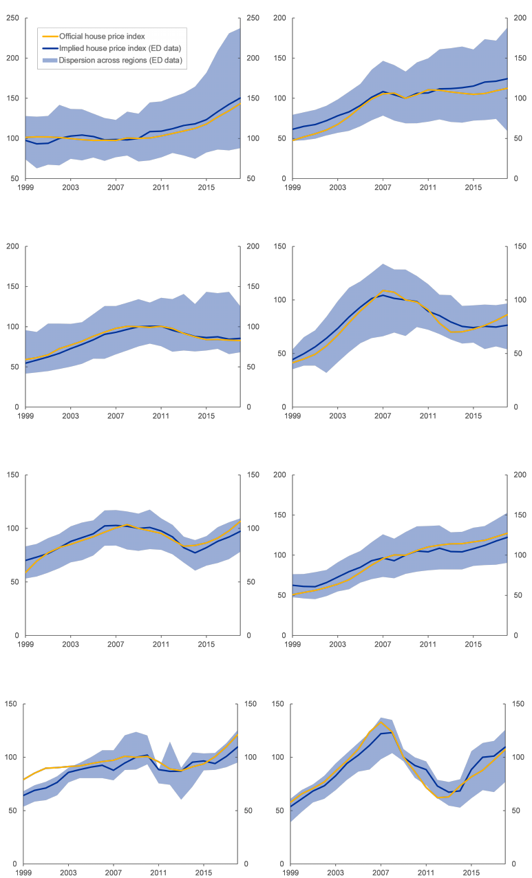
Figure A.2: House price indexes (2009=100)
(a) Germany (b) France
(c) Italy (d) Spain
(e) The Netherlands (f) Belgium
(g) Portugal (h) Ireland
ECB Working Paper Series No 2752 / November 2022
43

Figure A.3: Mortgage rates (in percentages per annum)
(a) Germany (b) France
(c) The Netherlands (d) Belgium
ECB Working Paper Series No 2752 / November 2022
44

Appendix B Additional tables and charts
Table B.1: Summary Statistics over sub-periods
Mean Median Minimum Maximum Standard Deviation
GDP 1999-2008 28923 28021 13786 66418 8844
GDP 2009-2012 29438 28133 14070 65112 9233
GDP 2013-2018 30394 28307 14914 65178 10368
Employment 1999-2008 43.86 43.08 31.31 65.43 6.68
Employment 2009-2012 43.48 42.78 31.55 66.83 7.06
Employment 2013-2018 43.33 42.24 30.15 68.23 7.36
House prices 1999-2008 132.89 129.02 93.25 187.27 22.32
House prices 2009-2012 163.03 164.57 93.44 233.93 34.34
House prices 2013-2018 156.51 156.57 104.69 237.29 26.20
Notes: Real GDP and employment are given in per capita terms. National GDP and employment are calculated
as cross-regional aggregate of all regions within a country. National house prices are given by GDP-weighted
cross-regional means of all regions within a country.
ECB Working Paper Series No 2752 / November 2022
45

Figure B.1: Monetary policy impact on house prices and regional factors
Notes: The y-axis reports the cumulative percentage change in (detrended) levels for house prices 5 years after
an accommodative monetary policy shock. The x-axis reports the regional housing wealth (thousand euros per
household), labour income (euros per employee, at 2015 prices), construction share (percent of value added), LTV
ratio (percent), share of variable-rate loans (percent of total loans). Each dot represents a region.
ECB Working Paper Series No 2752 / November 2022
46

Table B.2: Relationship between monetary policy impact on house prices and regional factors
(a) Dependent variable: (1) (2) (3) (4) (5) (6) (7) (8)
Impact of TMP shock
Compensation per employee -12.237*** -10.965*** -11.144*** -10.637*** -17.825**
Housing wealth 7.749*** 7.839** 7.189* 8.024
Homeownership rate 0.158***
House price level 7.093***
Share of construction in GVA 0.406 -0.297 -0.265 -0.433
Share of manufacturing in GVA 0.080 0.020 0.019 -0.004
Share of variable-rate mortgages 0.079*** 0.015 -0.011 -0.057
Lending activity 4.500*** -1.112 -0.687 -5.339
Demographics controls X X X X X X X X
Vulnerable dummy - - - - - - X -
Country dummies - - - - - - - X
Observations 105 105 105 105 105 105 105 105
R-squared 0.331 0.332 0.013 0.243 0.066 0.339 0.343 0.407
(b) Dependent variable: (1) (2) (3) (4) (5) (6) (7) (8)
Impact of CMP shock
Compensation per employee -5.918** -1.797 0.284 0.752 -21.486**
Housing wealth -1.780 -5.839 -6.439 9.553
Homeownership rate 0.080
House price level -7.738**
Share of construction in GVA 0.943* 0.325 0.354 -1.407
Share of manufacturing in GVA 0.101 0.080 0.078 0.046
Share of variable-rate mortgages 0.039** 0.046 0.022 -0.044
Lending activity -0.633 1.396 1.789 -8.752
Demographics controls X X X X X X X X
Vulnerable dummy - - - - - - X -
Country dummies - - - - - - - X
Observations 105 105 105 105 105 105 105 105
R-squared 0.067 0.109 0.052 0.062 0.023 0.098 0.100 0.187
(c) Dependent variable: (1) (2) (3) (4) (5) (6) (7) (8)
Impact of UMP shock
Compensation per employee -5.259** -10.905*** -19.487*** -19.834*** -10.680
Housing wealth 6.996*** 10.942*** 11.387*** 0.549
Homeownership rate -0.037
House price level 15.781***
Share of construction in GVA -0.747* -0.823* -0.845* -0.403
Share of manufacturing in GVA 0.063 0.077 0.078 0.084
Share of variable-rate mortgages 0.011 -0.104*** -0.086* -0.073
Lending activity 3.001* 1.364 1.072 3.703
Demographics controls X X X X X X X X
Vulnerable dummy - - - - - - X -
Country dummies - - - - - - - X
Observations 105 105 105 105 105 105 105 105
R-squared 0.171 0.301 0.071 0.036 0.061 0.342 0.344 0.418
Notes: The table present regressions of the cumulative monetary policy impact on house prices at the regional level (as estimated in
section 4) on regional factors (compensation per employee in logs, housing wealth in logs, homeownership rate in percent, the average
house price level in logs, the share of construction and manufacturing in GVA, the share of variable-rate mortgages in percent, and a
proxy for lending activity). Housing wealth is computed as the product of the homeownership rate and the average house price level.
The proxy for lending activity is computed as the product of housing wealth and the LTV ratio. Demographics controls include total
employment and population density at the regional level. The Vulnerable dummy is a binary variable that takes value one for regions
of Italy, Spain, Portugal and Ireland, and zero for regions of Germany, France, the Netherlands and Belgium. A constant is included.
An outlier is excluded. *** p <0.01, ** p<0.05, * p<0.1
ECB Working Paper Series No 2752 / November 2022
47

Figure B.2: Impulse response functions to an expansionary monetary policy shock - common
components
Notes: The y-axis reports the percentage change in (detrended) levels of each variable over the considered horizon.
The x-axis reports the years. This specification includes non-monetary policy common components. Solid lines
denote point estimates and light (dark) shaded areas 95 percent (68 percent) confidence bands.
ECB Working Paper Series No 2752 / November 2022
48
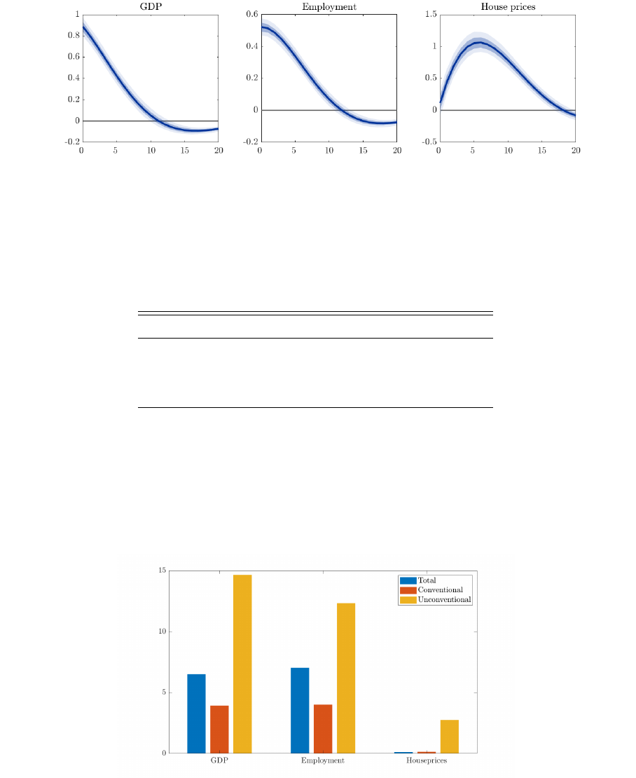
Figure B.3: Impulse response functions to an expansionary monetary policy shock - pooled
fixed-effect estimator
Notes: The y-axis reports the percentage change in (detrended) levels of each variable over the considered horizon.
The x-axis reports the years. These are the results of a fixed-effects regression. Solid lines denote point estimates
and light (dark) shaded areas 95 percent (68 percent) confidence bands.
Table B.3: Granger causality test results
GDP Employment House Prices
GDP / 0.000 0.005
Employment 0.269 / 0.010
House prices 0.143 0.587 /
Notes: The table shows the p-values of a Granger causality test. If the value in row i and column j is smaller
than 0.01 (0.05), then the null hypothesis that variable i does not Granger cause variable j has to be rejected at
the 1% (5%) significance level.
Figure B.4: Variance decomposition of key variables - alternative ordering
Notes: The y-axis reports the contribution of a total, conventional and unconventional monetary policy shock to
variations in GDP, employment and house prices at the 5-year horizon.
ECB Working Paper Series No 2752 / November 2022
49

Acknowledgements
We would like to thank Paola Di Casola, Simon Hildebrandt, Fédéric Holm-Hadulla, Bartosz Maćkowiak, Klaus Masuch, Beatrice
Pierluigi, Thomas Westermann and an anonymous referee for their helpful comments and suggestions. This paper has also benefitted
from discussions with participants at seminars at the ECB, the University of Bremen, the University of Neuchâtel, at the 6th Household
Finance Workshop (Leibniz Institute SAFE), at the 16
th
CEUS Workshop on European Economics, and at the 2022 ECHOPPE
Conference on the Economics of Housing and Housing Policies.
The views expressed in this paper are those of the authors and do not necessarily represent those of the European Central Bank.
Niccolò Battistini
European Central Bank, Frankfurt am Main, Germany; email: niccolo.battistini@ecb.europa.eu
Matteo Falagiarda
European Central Bank, Frankfurt am Main, Germany; email: matteo.falagiarda@ecb.europa.eu
Angelina Hackmann
University of Bremen, Bremen, Germany; email: angelina.hackmann@uni-bremen.de
Moreno Roma
European Central Bank, Frankfurt am Main, Germany; email: moreno.roma@ecb.europa.eu
© European Central Bank, 2022
Postal address 60640 Frankfurt am Main, Germany
Telephone +49 69 1344 0
Website www.ecb.europa.eu
All rights reserved. Any reproduction, publication and reprint in the form of a different publication, whether printed or produced
electronically, in whole or in part, is permitted only with the explicit written authorisation of the ECB or the authors.
This paper can be downloaded without charge from www.ecb.europa.eu, from the Social Science Research Network electronic library or
from RePEc: Research Papers in Economics. Information on all of the papers published in the ECB Working Paper Series can be found
on the ECB’s website.
PDF ISBN 978-92-899-5400-6 ISSN 1725-2806 doi:10.2866/439771 QB-AR-22-117-EN-N
